About this python module named tesseract, you can read here.
I tested with the tesseract tool install on my Fedora 30 distro and python module pytesseract version 0.3.0.
[root@desk mythcat]# dnf install tesseract
Last metadata expiration check: 0:24:18 ago on Sun 20 Oct 2019 10:56:23 AM EEST.
Package tesseract-4.1.0-1.fc30.x86_64 is already installed.
Dependencies resolved.
Nothing to do.
↧
Catalin George Festila: Python 3.7.4 : Usinge pytesseract for text recognition.
↧
Test and Code: 92: 9 Steps to Crater Quality & Destroy Customer Satisfaction - Cristian Medina
Cristian Medina wrote an article recently called "Test Engineering Anti-Patterns: Destroy Your Customer Satisfaction and Crater Your Quality By Using These 9 Easy Organizational Practices"
Of course, it's sarcastic, and aims to highlight many problems with organizational practices that reduce software quality.
The article doesn't go out of character, and only promotes the anti-patterns.
However, in this interview, we discuss each point, and the corollary of what you really should do. At least, our perspectives.
Here's the list of all the points discussed in the article and in this episode:
- Make the Test teams solely responsible for quality
- Require all tests to be automated before releasing
- Require 100% code coverage
- Isolate the Test organization from Development
- Measure the success of the process, not the product.
- Metrics, if rewarded, will always be gamed.
- Require granular projections from engineers
- Reward quick patching instead of solving
- Plan for today instead of tomorrow
Special Guest: Cristian Medina.
Sponsored By:
- Azure Pipelines: Automate your builds and deployments with pipelines so you spend less time with the nuts and bolts and more time being creative. Many organizations and open source projects are using Azure Pipelines already. Get started for free at azure.com/pipelines
Links:
- Test Engineering Anti-Patterns: Destroy Your Customer Satisfaction and Crater Your Quality By Using These 9 Easy Organizational Practices— The article we discuss in the show.
- tryexceptpass— Cris's blog
↧
↧
Kushal Das: tarted a newsletter
I started a newsletter, focusing on different stories I read about privacy, security, programming in general. Following the advice from Martijn Grooten, I am storing all the interesting links I read (for many months). I used to share these only over Twitter, but, as I retweet many things, it was not easy to share a selected few.
I also did not want to push them in my regular blog. I wanted a proper newsletter over email service. But, keeping the reader’s privacy was a significant point to choose the service. I finally decided to go with Write.as Letters service. I am already using their open source project WriteFreely. This is an excellent excuse to use their tool more and also pay them for the fantastic tools + service.
Feel free to subscribe to the newsletter and share the link with your friends.
↧
Go Deh: Indent datastructure for trees
I was browsing StackOverflow and came across a question that mentioned a new-to-me format for a datatructure for holding a tree of data.I am well used to the (name, list_of_children) set of interconnected node datastructures way of doing things, but this mentioned where you
![]()
1
2
4
7
5
3
6
8
9
10
![]()
![]()
- Create an empty list
- then for each node starting at the root which has a depth of zero:
- add the (depth, name) tuple of the node to the list
- visit all this nodes child node.
An example tree:

Its indent format:
[(0, 'R'),
 (1, 'a'),
 (2, 'c'),
 (3, 'd'),
 (3, 'h'),
 (1, 'b'),
 (2, 'e'),
 (3, 'f'),
 (4, 'g'),
 (2, 'i')]
Indented representation:
If you print out successive names from the indent format list above, one per line, with indent from the left of the indent value, then you get a nice textual regpresentation of the tree; expanded left-to-right rather than the top-down representation of the graphic:R
a
c
d
h
b
e
f
g
i
Code
I wrote some code to manipulate and traverse this kind of tree datastructure, as well as to use graphviz to draw graphical representations.1 | importgraphvizasgv |
Output:
A tree in indent datastructure format:
[(0, '1'),
(1, '2'),
(2, '4'),
(3, '7'),
(2, '5'),
(1, '3'),
(2, '6'),
(3, '8'),
(3, '9'),
(3, '10')]
Same tree, printed as indented list:
1
2
4
7
5
3
6
8
9
10
Same tree, drawn by graphviz:

Same tree, preorder traversal:
1 2 4 7 5 3 6 8 9 10
Same tree, levelorder traversal:
1 2 3 4 5 6 7 8 9 10
Same tree, reverse_depth levelorder traversal:
7 8 9 10 4 5 6 2 3 1
Same tree, reverse_depth, reverse_in_level levelorder traversal:
10 9 8 7 6 5 4 3 2 1
Same tree, depth_first, reverse_in_level levelorder traversal:
1 3 2 6 5 4 10 9 8 7
In [47]:
↧
Mike Driscoll: PyDev of the Week: Sophy Wong
This week we welcome Sophy Wong (@sophywong) as our PyDev of the Week! Sophy is a maker who uses Circuit Python for creating wearables. She is also a writer and speaker at Maker events. You can see some of her creations on her Youtube Channel or her website. Let’s take a few moments to get to know her better!

Can you tell us a little about yourself (hobbies, education, etc):
I am a designer and maker currently working mostly with wearable electronics projects. My background is in graphic design, and I have also worked in fashion and costumes on my way to wearable electronics. I like to explore the different ways people interact with technology, and much of my work is inspired by sci-fi and pop culture. My projects often combine technology, like microcontrollers and 3D printing, with hand crafts like sculpting, painting, and sewing.
Why did you start using Python?
I discovered Python through Adafruit’s development of Circuit Python. Adafruit’s thorough documentation and huge library of tutorial projects make it easy for me to learn and write code for my projects. I’m primarily a designer, and code is a tool I use to bring my ideas to life. Circuit Python helps me learn programming basics, and is also powerful enough to support more complex projects as I gain more skills.
What other programming languages do you know and which is your favorite?
I also use Arduino for some projects, which lets me use the many fantastic Arduino libraries out there, like FastLED. I often use MakeCode when creating a project for a tutorial or educational workshop. As a visual programming tool, MakeCode is intuitive to use and easy to explain with screenshots. It’s still robust enough to support fairly complex projects, and is a great first step before going further with Circuit Python or Arduino.
What projects are you working on now?
I recently completed a project that involved adding Adafruit’s NeoPixel RGB LEDs to a jacket, using 3D printed diffusers printed directly on fabric. I’m working on a project now that expands the technique to a larger, more elaborate garment. I’m also starting to work on another space suit concept, learning how to use a desktop PCB mill, and of course, writing more wearable tech project tutorials!
Which Python libraries are your favorite (core or 3rd party)?
Adafruit makes great Circuit Python libraries for all of their components, and I use their NeoPixel library for Circuit Python in almost every project, because I love making things light up with NeoPixels.
Do you have any advice for people who want to become makers?
Pick a project you’re really excited about and just start. Don’t wait for the perfect materials, or the fanciest tools, get scrappy and figure it out as you go. Sometimes too much planning and preparation can steal all your energy before you ever get going, and make your project feel overwhelming. So fall in love with your idea, and jump in while you’re excited. Trust yourself, and have fun. You can’t fail if you never give up!
What new wearable tech are you excited about?
I’m really excited about VR and the potential for wearables to add to the immersive experience. It’s a technology I remember being amazed by when I was a kid. I really wanted to try it, but the technology was so far out of reach for me, I thought I’d never be able to experience it myself. Now that it’s available as consumer technology, I’m very interested to see makers create their own VR experiences, as well as wearable devices and peripherals for VR.
I’m also very interested in space exploration and space suits. I’ve made my own space suit costume, a conceptual design that is based on sci-fi renderings. With upcoming missions to the Moon and Mars, I’m excited to see innovations in space suit design, and how designers and engineers create new suits for both astronauts and space tourists.
Is there anything else you’d like to say?
Thank you to everyone who documents their projects and shares their work for others to learn from! Thanks to tutorials and libraries written and published by others, I’m able to bring my ideas to life with programmable electronics. I never thought that studying design would lead me to learning how to code, and writing tutorials to help others get started with programming. Now, writing Circuit Python code for my projects is one of my favorite parts of the process!
Thanks for doing the interview, Sophy!
The post PyDev of the Week: Sophy Wong appeared first on The Mouse Vs. The Python.
↧
↧
Erik Marsja: Converting HTML to a Jupyter Notebook
The post Converting HTML to a Jupyter Notebook appeared first on Erik Marsja.
In this short post, we are going to learn how to turn the code from blog posts to Jupyter notebooks.
In this post, we are going to use the Python packages BeautifulSoup4, json, and urllib. We are going to use these packages to scrape the code from webpages putting their code within <code></code>.
Note, this code is not intended to steal other people’s code. I created this script to scrape my code and save it to Jupyter notebooks because I noticed that my code, sometimes did not work as intended.
Install the Needed Packages
Now, we need to install BeautifulSoup4 before we continue converting html
to jupyter notebooks. Furthermore, we need to install lxml.
How to Install Python Packages using conda
In this section, we are going to learn how to install the needed packages using the packages manager conda. First, open up the Anaconda Powershell Prompt
Now, we are ready to install BeautifulSoup4.
conda -c install anaconda beautifulsoup4 lxmlHow to Install Python Packages using Pip
It is, of course, possible to install the packages using pip as well:
install beautifulsoup4 lxmlHow to Convert HTML to a Jupyter Notebook
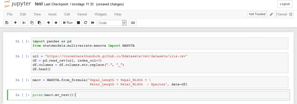
Now, when we have installed the Python packages, we can continue with scraping the code from a web page. In the example, below, we will start by importing BeautifulSoup from bs4, json, and urllib. Next, we have the URL to the webpage that we want to convert to a Jupyter notebooks (this).
from bs4 import BeautifulSoup
  import json
  import urllib

  url = 'https://www.marsja.se/python-manova-made-easy-using-statsmodels/'
Setting a Custom User-Agent
In the next line of code, we create the dictionary headers.
This is because many websites (including the one you are reading now) will block web scrapers and this will prevent that from happening.
  headers = {'User-Agent': 'Mozilla/5.0 (X11; Linux x86_64) AppleWebKit/537.11'\
             '(KHTML, like Gecko) Chrome/23.0.1271.64 Safari/537.11',
         'Accept': 'text/html,application/xhtml+xml,application/xml;q=0.9,*/*;q=0.8',
         'Accept-Charset': 'ISO-8859-1,utf-8;q=0.7,*;q=0.3',
         'Accept-Encoding': 'none',
         'Accept-Language': 'en-US,en;q=0.8',
         'Connection': 'keep-alive'}
In the next code chunk, we are going to create a Request object. This object represents the HTTP request we are making.
Simply put, we create a Request object that specifies the URL we want to retrieve. Furthermore, we are calling urlopen using the Request object. This will, in turn, a response object for the requested URL.
Finally, we call .read() on the response:
req = urllib.request.Request(url,
    headers=headers)
  page = urllib.request.urlopen(req)
  text = page.read()
We are now going to use BeautifulSoup4 to get make it easier to scrape the html:
soup = BeautifulSoup(text, 'lxml')
soup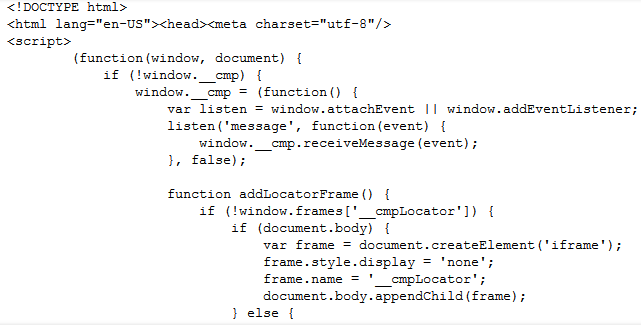
Jupyter Notebook Metadata
Now we’re ready to convert HTML to a Jupyter Notebook (this code was inspired by this code example). First, we start by creating some metadata for the Jupyter notebook.
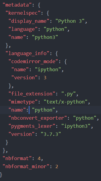 Jupyter notebook metadata
In the code below, we start by creating a dictionary in which we will, later, store our scraped code elements. This is going to be the metadata for the Jupyter notebook we will create. Note, .ipynb are simple JSON files, containing text, code, rich media output, and metadata. The metadata is not required but here we will add what language we are using (i.e., Python 3).
create_nb = {'nbformat': 4, 'nbformat_minor': 2,
'cells': [], 'metadata':
{"kernelspec":
{"display_name": "Python 3",
"language": "python", "name": "python3"
}}}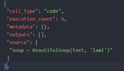 Example code cell from a Jupyter Notebook
More information bout the format of Jupyter notebooks can be found here.
Getting the Code Elements from the HTML
Second, we are creating a Python function called get_code. This function will take two arguments. First, the beautifulsoup object, we earlier created, and the content_class to search for content in. In the case, of this particular WordPress, blog this will be post-content
Next, we are looping through all div tags in the soup object. Here, we only look for the post content. Next, we get all the code chunks searching for all code tags
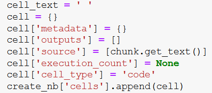
In the final loop, we are going through each code chunk and creating a new dictionary (cell) in which we are going to store the code. The important part is where we add the text, using the get_text method. Here we are getting our code from the code chunk and add it to the dictionary.
Finally, we add this to the dictionary, nb_data, that will contain the data that we are going to save as a jupyter notebook (i.e., the blog post we have scraped).
def get_data(soup, content_class):
    for div in soup.find_all('div',
                             attrs={'class': content_class}):

        code_chunks = div.find_all('code')

        for chunk in code_chunks:
            cell_text = ' '
            cell = {}
            cell['metadata'] = {}
            cell['outputs'] = []
            cell['source'] = [chunk.get_text()]
            cell['execution_count'] = None
            cell['cell_type'] = 'code'
            create_nb['cells'].append(cell)

get_data(soup, 'post-content')

with open('Python_MANOVA.ipynb', 'w') as jynotebook:
jynotebook.write(json.dumps(create_nb))- More about parsing JSON in Python
Note, we get the nb_data which is a dictionary from which will create our notebook from. In the final two rows, of the code chunk, we will open a file (i.e., test.ipynb) and write to this file using json dump method.
Here’s a Jupyter notebook containing all code above.
The post Converting HTML to a Jupyter Notebook appeared first on Erik Marsja.
↧
Anwesha Das: CopyleftConf 2020
A week before Software Freedom Conservancy had announced the CopyleftConf 2020. The conference is going to take place on 3 February 2020, Monday, in Brussels, Belgium.
The first edition of CopyleftConf took place in February 2019. One can have a look at the videos here The organizers do plan it after Fosdem.
This is a unique conference that assembles the copyleft community around the globe.
There will be a comprehensive and thorough discussion of various topics. Which includes daily beginner level to expert level issues, stuff related to copyright licensing, challenges faced by the programmers to license their code under copyleft licenses. The developers, strategists, enforcement organizations, scholars, and critics take part in the conference.
One of the primary aim of the conference is having an extensive discussion on the “obstacles facing copyleft and the future of copyleft as a strategy to advance and defend software freedom for users and developers around the world.” This is a dream come true conference for all the Copyleft followers and believers.
The call for proposal is open. And it will be open till 3rd November 2019, midnight AOE. They are welcoming talks for the duration of 20 minutes + 5 minutes QA, or if you want to speak for the whole 25 minutes, that is also welcome.
The organizers are also welcoming proposals for an hour-long discussion. The facilitators will introduce the topic in the first 5 to 10 minutes. They are free to decide on the format. People are asked to submit a proposal in groups or pairs. The organizers are interested in having people having different perspectives, viewpoints on the subject, being the facilitators of the discussion.
At the end of the discussion, there should be some functional ideas for "better use and increased adoption of copylefted software. "
People are asked to submit proposals on and around the topics mentioned above. Some of the example fields and issues being:
- Governance concerns for large copyleft projects;
- Social and/or technical compliance strategies;
- How copyleft fits in with other efforts to build ethical technology;
- Is it possible or desirable to include ethical considerations beyond software freedom into FOSS licenses?
- Copyleft and enforcement in different jurisdictions;
- Affero GPL and other copyleft considerations in the era of network-based service software;
- Publicly funded copyleft; i.e. municipal, library, public school or government;
- License compatibility, what's new, what's old, and what challenges remain?
- Copyleft abuse, how should the community respond?
- The (general) future of copyleft;
- any other topic (which is not on the list) that relates to copyleft.
If one is unsure about the proposal being good enough for the conference, can ask for help.
The organizers are available in the #conservancy IRC channel on freenode, mail them, or twitter is another option.
I very much want to be there and take part in the conference but not sure if geographical distance will allow me to do it or not. But surely will be attending the conference through the live recording (hopefully the organizers will have it this year as well).
If you are a complete beginner and want to know about Copyleft, I urge you to be a part of this conference. Please do not be intimidated by the names of people attending it. They are the most helpful and friendly human beings you will ever find (quoting this from my personal experience). And now, when you have the time and chance to know "what is Copyleft?", from the best, then why not :).
Therefore book your dates for the conference and see you there.
↧
qutebrowser development blog: Current qutebrowser roadmap and next crowdfunding
More than half a year ago, I posted a qutebrowser roadmap - I thought it's about time for an update on how things are looking at the moment!
Upcoming crowdfunding
I finished my Bachelor of Science in September at the University of Applied Sciences in Rapperswil.
Now I'm employed around 16h …
↧
Real Python: Arduino With Python: How to Get Started
Microcontrollers have been around for a long time, and they’re used in everything from complex machinery to common household appliances. However, working with them has traditionally been reserved for those with formal technical training, such as technicians and electrical engineers. The emergence of Arduino has made electronic application design much more accessible to all developers. In this tutorial, you’ll discover how to use Arduino with Python to develop your own electronic projects.
You’ll cover the basics of Arduino with Python and learn how to:
- Set up electronic circuits
- Set up the Firmata protocol on Arduino
- Write basic applications for Arduino in Python
- Control analog and digital inputs and outputs
- Integrate Arduino sensors and switches with higher-level apps
- Trigger notifications on your PC and send emails using Arduino
Free Bonus:5 Thoughts On Python Mastery, a free course for Python developers that shows you the roadmap and the mindset you'll need to take your Python skills to the next level.
The Arduino Platform
Arduino is an open-source platform composed of hardware and software that allows for the rapid development of interactive electronics projects. The emergence of Arduino drew the attention of professionals from many different industries, contributing to the start of the Maker Movement.
With the growing popularity of the Maker Movement and the concept of the Internet of Things, Arduino has become one of the main platforms for electronic prototyping and the development of MVPs.
Arduino uses its own programming language, which is similar to C++. However, it’s possible to use Arduino with Python or another high-level programming language. In fact, platforms like Arduino work well with Python, especially for applications that require integration with sensors and other physical devices.
All in all, Arduino and Python can facilitate an effective learning environment that encourages developers to get into electronics design. If you already know the basics of Python, then you’ll be able to get started with Arduino by using Python to control it.
The Arduino platform includes both hardware and software products. In this tutorial, you’ll use Arduino hardware and Python software to learn about basic circuits, as well as digital and analog inputs and outputs.
Arduino Hardware
To run the examples, you’ll need to assemble the circuits by hooking up electronic components. You can generally find these items at electronic component stores or in good Arduino starter kits. You’ll need:
- An Arduino Uno or other compatible board
- A standard LED of any color
- A push button
- A 10 KOhm potentiometer
- A 470 Ohm resistor
- A 10 KOhm resistor
- A breadboard
- Jumper wires of various colors and sizes
Let’s take a closer look at a few of these components.
Component 1 is an Arduino Uno or other compatible board. Arduino is a project that includes many boards and modules for different purposes, and Arduino Uno is the most basic among these. It’s also the most used and most documented board of the whole Arduino family, so it’s a great choice for developers who are just getting started with electronics.
Note: Arduino is an open hardware platform, so there are many other vendors who sell compatible boards that could be used to run the examples you see here. In this tutorial, you’ll learn how to use the Arduino Uno.
Components 5 and 6 are resistors. Most resistors are identified by colored stripes according to a color code. In general, the first three colors represent the value of a resistor, while the fourth color represents its tolerance. For a 470 Ohm resistor, the first three colors are yellow, violet, and brown. For a 10 KOhm resistor, the first three colors are brown, black, and orange.
Component 7 is a breadboard, which you use to hook up all the other components and assemble the circuits. While a breadboard is not required, it’s recommended that you get one if you intend to begin working with Arduino.
Arduino Software
In addition to these hardware components, you’ll need to install some software. The platform includes the Arduino IDE, an Integrated Development Environment for programming Arduino devices, among other online tools.
Arduino was designed to allow you to program the boards with little difficulty. In general, you’ll follow these steps:
- Connect the board to your PC
- Install and open the Arduino IDE
- Configure the board settings
- Write the code
- Press a button on the IDE to upload the program to the board
To install the Arduino IDE on your computer, download the appropriate version for your operating system from the Arduino website. Check the documentation for installation instructions:
- If you’re using Windows, then use the Windows installer to ensure you download the necessary drivers for using Arduino on Windows. Check the Arduino documentation for more details.
- If you’re using Linux, then you may have to add your user to some groups in order to use the serial port to program Arduino. This process is described in the Arduino install guide for Linux.
- If you’re using macOS, then you can install Arduino IDE by following the Arduino install guide for OS X.
Note: You’ll be using the Arduino IDE in this tutorial, but Arduino also provides a web editor that will let you program Arduino boards using the browser.
Now that you’ve installed the Arduino IDE and gathered all the necessary components, you’re ready to get started with Arduino! Next, you’ll upload a “Hello, World!” program to your board.
“Hello, World!” With Arduino
The Arduino IDE comes with several example sketches you can use to learn the basics of Arduino. A sketch is the term you use for a program that you can upload to a board. Since the Arduino Uno doesn’t have an attached display, you’ll need a way to see the physical output from your program. You’ll use the Blink example sketch to make a built-in LED on the Arduino board blink.
Uploading the Blink Example Sketch
To get started, connect the Arduino board to your PC using a USB cable and start the Arduino IDE. To open the Blink example sketch, access the File menu and select Examples, then 01.Basics and, finally, Blink:

The Blink example code will be loaded into a new IDE window. But before you can upload the sketch to the board, you’ll need to configure the IDE by selecting your board and its connected port.
To configure the board, access the Tools menu and then Board. For Arduino Uno, you should select Arduino/Genuino Uno:

After you select the board, you have to set the appropriate port. Access the Tools menu again, and this time select Port:

The names of the ports may be different, depending on your operating system. In Windows, the ports will be named COM4, COM5, or something similar. In macOS or Linux, you may see something like /dev/ttyACM0 or /dev/ttyUSB0. If you have any problems setting the port, then take a look at the Arduino Troubleshooting Page.
After you’ve configured the board and port, you’re all set to upload the sketch to your Arduino. To do that, you just have to press the Upload button in the IDE toolbar:

When you press Upload, the IDE compiles the sketch and uploads it to your board. If you want to check for errors, then you can press Verify before Upload, which will only compile your sketch.
The USB cable provides a serial connection to both upload the program and power the Arduino board. During the upload, you’ll see LEDs flashing on the board. After a few seconds, the uploaded program will run, and you’ll see an LED light blink once every second:

After the upload is finished, the USB cable will continue to power the Arduino board. The program is stored in flash memory on the Arduino microcontroller. You can also use a battery or other external power supply to run the application without a USB cable.
Connecting External Components
In the previous section, you used an LED that was already present on the Arduino board. However, in most practical projects you’ll need to connect external components to the board. To make these connections, Arduino has several pins of different types:

Although these connections are commonly called pins, you can see that they’re not exactly physical pins. Rather, the pins are holes in a socket to which you can connect jumper wires. In the figure above, you can see different groups of pins:
- Orange rectangle: These are 13 digital pins that you can use as inputs or outputs. They’re only meant to work with digital signals, which have 2 different levels:
- Level 0: represented by the voltage 0V
- Level 1: represented by the voltage 5V
- Green rectangle: These are 6 analog pins that you can use as analog inputs. They’re meant to work with an arbitrary voltage between 0V and 5V.
- Blue rectangle: These are 5 power pins. They’re mainly used for powering external components.
To get started using external components, you’ll connect an external LED to run the Blink example sketch. The built-in LED is connected to digital pin #13. So, let’s connect an external LED to that pin and check if it blinks. (A standard LED is one of the components you saw listed earlier.)
Before you connect anything to the Arduino board, it’s good practice to disconnect it from the computer. With the USB cable unplugged, you’ll be able to connect the LED to your board:

Note that the figure shows the board with the digital pins now facing you.
Using a Breadboard
Electronic circuit projects usually involve testing several ideas, with you adding new components and making adjustments as you go. However, it can be tricky to connect components directly, especially if the circuit is large.
To facilitate prototyping, you can use a breadboard to connect the components. This is a device with several holes that are connected in a particular way so that you can easily connect components using jumper wires:

You can see which holes are interconnected by looking at the colored lines. You’ll use the holes on the sides of the breadboard to power the circuit:
- Connect one hole on the red line to the power source.
- Connect one hole on the blue line to the ground.
Then, you can easily connect components to the power source or the ground by simply using the other holes on the red and blue lines. The holes in the middle of the breadboard are connected as indicated by the colors. You’ll use these to make connections between the components of the circuit. These two internal sections are separated by a small depression, over which you can connect integrated circuits (ICs).
You can use a breadboard to assemble the circuit used in the Blink example sketch:

For this circuit, it’s important to note that the LED must be connected according to its polarity or it won’t work. The positive terminal of the LED is called the anode and is generally the longer one. The negative terminal is called the cathode and is shorter. If you’re using a recovered component, then you can also identify the terminals by looking for a flat side on the LED itself. This will indicate the position of the negative terminal.
When you connect an LED to an Arduino pin, you’ll always need a resistor to limit its current and avoid burning out the LED prematurely. Here, you use a 470 Ohm resistor to do this. You can follow the connections and check that the circuit is the same:
- The resistor is connected to digital pin 13 on the Arduino board.
- The LED anode is connected to the other terminal of the resistor.
- The LED cathode is connected to the ground (GND) via the blue line of holes.
For a more detailed explanation, check out How to Use a Breadboard.
After you finish the connection, plug the Arduino back into the PC and re-run the Blink sketch:

As both LEDs are connected to digital pin 13, they blink together when the sketch is running.
“Hello, World!” With Arduino and Python
In the previous section, you uploaded the Blink sketch to your Arduino board. Arduino sketches are written in a language similar to C++ and are compiled and recorded on the flash memory of the microcontroller when you press Upload. While you can use another language to directly program the Arduino microcontroller, it’s not a trivial task!
However, there are some approaches you can take to use Arduino with Python or other languages. One idea is to run the main program on a PC and use the serial connection to communicate with Arduino through the USB cable. The sketch would be responsible for reading the inputs, sending the information to the PC, and getting updates from the PC to update the Arduino outputs.
To control Arduino from the PC, you’d have to design a protocol for the communication between the PC and Arduino. For example, you could consider a protocol with messages like the following:
- VALUE OF PIN 13 IS HIGH: used to tell the PC about the status of digital input pins
- SET PIN 11 LOW: used to tell Arduino to set the states of the output pins
With the protocol defined, you could write an Arduino sketch to send messages to the PC and update the states of the pins according to the protocol. On the PC, you could write a program to control the Arduino through a serial connection, based on the protocol you’ve designed. For this, you can use whatever language and libraries you prefer, such as Python and the PySerial library.
Fortunately, there are standard protocols to do all this! Firmata is one of them. This protocol establishes a serial communication format that allows you to read digital and analog inputs, as well as send information to digital and analog outputs.
The Arduino IDE includes ready-made sketches that will drive Arduino through Python with the Firmata protocol. On the PC side, there are implementations of the protocol in several languages, including Python. To get started with Firmata, let’s use it to implement a “Hello, World!” program.
Uploading the Firmata Sketch
Before you write your Python program to drive Arduino, you have to upload the Firmata sketch so that you can use that protocol to control the board. The sketch is available in the Arduino IDE’s built-in examples. To open it, access the File menu, then Examples, followed by Firmata, and finally StandardFirmata:

The sketch will be loaded into a new IDE window. To upload it to the Arduino, you can follow the same steps you did before:
- Plug the USB cable into the PC.
- Select the appropriate board and port on the IDE.
- Press Upload.
After the upload is finished, you won’t notice any activity on the Arduino. To control it, you still need a program that can communicate with the board through the serial connection. To work with the Firmata protocol in Python, you’ll need the pyFirmata package, which you can install with pip:
$ pip install pyfirmata
After the installation finishes, you can run an equivalent Blink application using Python and Firmata:
1 importpyfirmata 2 importtime 3 4 board=pyfirmata.Arduino('/dev/ttyACM0') 5 6 whileTrue: 7 board.digital[13].write(1) 8 time.sleep(1) 9 board.digital[13].write(0)10 time.sleep(1)Here’s how this program works. You import pyfirmata and use it to establish a serial connection with the Arduino board, which is represented by the board object in line 4. You also configure the port in this line by passing an argument to pyfirmata.Arduino(). You can use the Arduino IDE to find the port.
board.digital is a list whose elements represent the digital pins of the Arduino. These elements have the methods read() and write(), which will read and write the state of the pins. Like most embedded device programs, this program mainly consists of an infinite loop:
- In line 7, digital pin 13 is turned on, which turns the LED on for one second.
- In line 9, this pin is turned off, which turns the LED off for one second.
Now that you know the basics of how to control an Arduino with Python, let’s go through some applications to interact with its inputs and outputs.
Reading Digital Inputs
Digital inputs can have only two possible values. In a circuit, each of these values is represented by a different voltage. The table below shows the digital input representation for a standard Arduino Uno board:
| Value | Level | Voltage |
|---|---|---|
| 0 | Low | 0V |
| 1 | High | 5V |
To control the LED, you’ll use a push button to send digital input values to the Arduino. The button should send 0V to the board when it’s released and 5V to the board when it’s pressed. The figure below shows how to connect the button to the Arduino board:

You may notice that the LED is connected to the Arduino on digital pin 13, just like before. Digital pin 10 is used as a digital input. To connect the push button, you have to use the 10 KOhm resistor, which acts as a pull down in this circuit. A pull down resistor ensures that the digital input gets 0V when the button is released.
When you release the button, you open the connection between the two wires on the button. Since there’s no current flowing through the resistor, pin 10 just connects to the ground (GND). The digital input gets 0V, which represents the 0 (or low) state. When you press the button, you apply 5V to both the resistor and the digital input. A current flows through the resistor and the digital input gets 5V, which represents the 1 (or high) state.
You can use a breadboard to assemble the above circuit as well:

Now that you’ve assembled the circuit, you have to run a program on the PC to control it using Firmata. This program will turn on the LED, based on the state of the push button:
1 importpyfirmata 2 importtime 3 4 board=pyfirmata.Arduino('/dev/ttyACM0') 5 6 it=pyfirmata.util.Iterator(board) 7 it.start() 8 9 board.digital[10].mode=pyfirmata.INPUT10 11 whileTrue:12 sw=board.digital[10].read()13 ifswisTrue:14 board.digital[13].write(1)15 else:16 board.digital[13].write(0)17 time.sleep(0.1)Let’s walk through this program:
- Lines 1 and 2 import
pyfirmataandtime. - Line 4 uses
pyfirmata.Arduino()to set the connection with the Arduino board. - Line 6 assigns an iterator that will be used to read the status of the inputs of the circuit.
- Line 7 starts the iterator, which keeps a loop running in parallel with your main code. The loop executes
board.iterate()to update the input values obtained from the Arduino board. - Line 9 sets pin 10 as a digital input with
pyfirmata.INPUT. This is necessary since the default configuration is to use digital pins as outputs. - Line 11 starts an infinite
whileloop. This loop reads the status of the input pin, stores it insw, and uses this value to turn the LED on or off by changing the value of pin 13. - Line 17 waits 0.1 seconds between iterations of the
whileloop. This isn’t strictly necessary, but it’s a nice trick to avoid overloading the CPU, which reaches 100% load when there isn’t a wait command in the loop.
pyfirmata also offers a more compact syntax to work with input and output pins. This may be a good option for when you’re working with several pins. You can rewrite the previous program to have more compact syntax:
1 importpyfirmata 2 importtime 3 4 board=pyfirmata.Arduino('/dev/ttyACM0') 5 6 it=pyfirmata.util.Iterator(board) 7 it.start() 8 9 digital_input=board.get_pin('d:10:i')10 led=board.get_pin('d:13:o')11 12 whileTrue:13 sw=digital_input.read()14 ifswisTrue:15 led.write(1)16 else:17 led.write(0)18 time.sleep(0.1)In this version, you use board.get_pin() to create two objects. digital_input represents the digital input state, and led represents the LED state. When you run this method, you have to pass a string argument composed of three elements separated by colons:
- The type of the pin (
afor analog ordfor digital) - The number of the pin
- The mode of the pin (
ifor input orofor output)
Since digital_input is a digital input using pin 10, you pass the argument 'd:10:i'. The LED state is set to a digital output using pin 13, so the led argument is 'd:13:o'.
When you use board.get_pin(), there’s no need to explicitly set up pin 10 as an input like you did before with pyfirmata.INPUT. After the pins are set, you can access the status of a digital input pin using read(), and set the status of a digital output pin with write().
Digital inputs are widely used in electronics projects. Several sensors provide digital signals, like presence or door sensors, that can be used as inputs to your circuits. However, there are some cases where you’ll need to measure analog values, such as distance or physical quantities. In the next section, you’ll see how to read analog inputs using Arduino with Python.
Reading Analog Inputs
In contrast to digital inputs, which can only be on or off, analog inputs are used to read values in some range. On the Arduino Uno, the voltage to an analog input ranges from 0V to 5V. Appropriate sensors are used to measure physical quantities, such as distances. These sensors are responsible for encoding these physical quantities in the proper voltage range so they can be read by the Arduino.
To read an analog voltage, the Arduino uses an analog-to-digital converter (ADC), which converts the input voltage to a digital number with a fixed number of bits. This determines the resolution of the conversion. The Arduino Uno uses a 10-bit ADC and can determine 1024 different voltage levels.
The voltage range for an analog input is encoded to numbers ranging from 0 to 1023. When 0V is applied, the Arduino encodes it to the number 0. When 5V is applied, the encoded number is 1023. All intermediate voltage values are proportionally encoded.
A potentiometer is a variable resistor that you can use to set the voltage applied to an Arduino analog input. You’ll connect it to an analog input to control the frequency of a blinking LED:

In this circuit, the LED is set up just as before. The end terminals of the potentiometer are connected to ground (GND) and 5V pins. This way, the central terminal (the cursor) can have any voltage in the 0V to 5V range depending on its position, which is connected to the Arduino on analog pin A0.
Using a breadboard, you can assemble this circuit as follows:

Before you control the LED, you can use the circuit to check the different values the Arduino reads, based on the position of the potentiometer. To do this, run the following program on your PC:
1 importpyfirmata 2 importtime 3 4 board=pyfirmata.Arduino('/dev/ttyACM0') 5 it=pyfirmata.util.Iterator(board) 6 it.start() 7 8 analog_input=board.get_pin('a:0:i') 9 10 whileTrue:11 analog_value=analog_input.read()12 print(analog_value)13 time.sleep(0.1)In line 8, you set up analog_input as the analog A0 input pin with the argument 'a:0:i'. Inside the infinite while loop, you read this value, store it in analog_value, and display the output to the console with print(). When you move the potentiometer while the program runs, you should output similar to this:
0.00.02930.10560.18380.27170.37050.44280.50640.57970.63150.67640.72430.78590.84460.90420.96771.01.0The printed values change, ranging from 0 when the position of the potentiometer is on one end to 1 when it’s on the other end. Note that these are float values, which may require conversion depending on the application.
To change the frequency of the blinking LED, you can use the analog_value to control how long the LED will be kept on or off:
1 importpyfirmata 2 importtime 3 4 board=pyfirmata.Arduino('/dev/ttyACM0') 5 it=pyfirmata.util.Iterator(board) 6 it.start() 7 8 analog_input=board.get_pin('a:0:i') 9 led=board.get_pin('d:13:o')10 11 whileTrue:12 analog_value=analog_input.read()13 ifanalog_valueisnotNone:14 delay=analog_value+0.0115 led.write(1)16 time.sleep(delay)17 led.write(0)18 time.sleep(delay)19 else:20 time.sleep(0.1)Here, you calculate delay as analog_value + 0.01 to avoid having delay equal to zero. Otherwise, it’s common to get an analog_value of None during the first few iterations. To avoid getting an error when running the program, you use a conditional in line 13 to test whether analog_value is None. Then you control the period of the blinking LED.
Try running the program and changing the position of the potentiometer. You’ll notice the frequency of the blinking LED changes:

By now, you’ve seen how to use digital inputs, digital outputs, and analog inputs on your circuits. In the next section, you’ll see how to use analog outputs.
Using Analog Outputs
In some cases, it’s necessary to have an analog output to drive a device that requires an analog signal. Arduino doesn’t include a real analog output, one where the voltage could be set to any value in a certain range. However, Arduino does include several Pulse Width Modulation (PWM) outputs.
PWM is a modulation technique in which a digital output is used to generate a signal with variable power. To do this, it uses a digital signal of constant frequency, in which the duty cycle is changed according to the desired power. The duty cycle represents the fraction of the period in which the signal is set to high.
Not all Arduino digital pins can be used as PWM outputs. The ones that can be are identified by a tilde (~):

Several devices are designed to be driven by PWM signals, including some motors. It’s even possible to obtain a real analog signal from the PWM signal if you use analog filters. In the previous example, you used a digital output to turn an LED light on or off. In this section, you’ll use PWM to control the brightness of an LED, according to the value of an analog input given by a potentiometer.
When a PWM signal is applied to an LED, its brightness varies according to the duty cycle of the PWM signal. You’re going to use the following circuit:

This circuit is identical to the one used in the previous section to test the analog input, except for one difference. Since it’s not possible to use PWM with pin 13, the digital output pin used for the LED is pin 11.
You can use a breadboard to assemble the circuit as follows:

With the circuit assembled, you can control the LED using PWM with the following program:
1 importpyfirmata 2 importtime 3 4 board=pyfirmata.Arduino('/dev/ttyACM0') 5 6 it=pyfirmata.util.Iterator(board) 7 it.start() 8 9 analog_input=board.get_pin('a:0:i')10 led=board.get_pin('d:11:p')11 12 whileTrue:13 analog_value=analog_input.read()14 ifanalog_valueisnotNone:15 led.write(analog_value)16 time.sleep(0.1)There are a few differences from the programs you’ve used previously:
- In line 10, you set
ledto PWM mode by passing the argument'd:11:p'. - In line 15, you call
led.write()withanalog_valueas an argument. This is a value between 0 and 1, read from the analog input.
Here you can see the LED behavior when the potentiometer is moved:

To show the changes in the duty cycle, an oscilloscope is plugged into pin 11. When the potentiometer is in its zero position, you can see the LED is turned off, as pin 11 has 0V on its output. As you turn the potentiometer, the LED gets brighter as the PWM duty cycle increases. When you turn the potentiometer all the way, the duty cycle reaches 100%. The LED is turned on continuously at maximum brightness.
With this example, you’ve covered the basics of using an Arduino and its digital and analog inputs and outputs. In the next section, you’ll see an application for using Arduino with Python to drive events on the PC.
Using a Sensor to Trigger a Notification
Firmata is a nice way to get started with Arduino with Python, but the need for a PC or other device to run the application can be costly, and this approach may not be practical in some cases. However, when it’s necessary to collect data and send it to a PC using external sensors, Arduino and Firmata make a good combination.
In this section, you’ll use a push button connected to your Arduino to mimic a digital sensor and trigger a notification on your machine. For a more practical application, you can think of the push button as a door sensor that will trigger an alarm notification, for example.
To display the notification on the PC, you’re going to use Tkinter, the standard Python GUI toolkit. This will show a message box when you press the button. For an in-depth intro to Tkinter, check out the library’s documentation.
You’ll need to assemble the same circuit that you used in the digital input example:
After you assemble the circuit, use the following program to trigger the notifications:
1 importpyfirmata 2 importtime 3 importtkinter 4 fromtkinterimportmessagebox 5 6 root=tkinter.Tk() 7 root.withdraw() 8 9 board=pyfirmata.Arduino('/dev/ttyACM0')10 11 it=pyfirmata.util.Iterator(board)12 it.start()13 14 digital_input=board.get_pin('d:10:i')15 led=board.get_pin('d:13:o')16 17 whileTrue:18 sw=digital_input.read()19 ifswisTrue:20 led.write(1)21 messagebox.showinfo("Notification","Button was pressed")22 root.update()23 led.write(0)24 time.sleep(0.1)This program is similar to the one used in the digital input example, with a few changes:
- Lines 3 and 4 import libraries needed to set up Tkinter.
- Line 6 creates Tkinter’s main window.
- Line 7 tells Tkinter not to show the main window on the screen. For this example, you only need to see the message box.
- Line 17 starts the
whileloop:- When you press the button, the LED will turn on and
messagebox.showinfo()displays a message box. - The loop pauses until the user presses OK. This way, the LED remains on as long as the message is on the screen.
- After the user presses OK,
root.update()clears the message box from the screen and the LED is turned off.
- When you press the button, the LED will turn on and
To extend the notification example, you could even use the push button to send an email when pressed:
1 importpyfirmata 2 importtime 3 importsmtplib 4 importssl 5 6 defsend_email(): 7 port=465# For SSL 8 smtp_server="smtp.gmail.com" 9 sender_email="<your email address>"10 receiver_email="<destination email address>"11 password="<password>"12 message="""Subject: Arduino Notification\n The switch was turned on."""13 14 context=ssl.create_default_context()15 withsmtplib.SMTP_SSL(smtp_server,port,context=context)asserver:16 print("Sending email")17 server.login(sender_email,password)18 server.sendmail(sender_email,receiver_email,message)19 20 board=pyfirmata.Arduino('/dev/ttyACM0')21 22 it=pyfirmata.util.Iterator(board)23 it.start()24 25 digital_input=board.get_pin('d:10:i')26 27 whileTrue:28 sw=digital_input.read()29 ifswisTrue:30 send_email()31 time.sleep(0.1)You can learn more about send_email() in Sending Emails With Python. Here, you configure the function with email server credentials, which will be used to send the email.
Note: If you use a Gmail account to send the emails, then you need to enable the Allow less secure apps option. For more information on how to do this, check out Sending Emails With Python.
With these example applications, you’ve seen how to use Firmata to interact with more complex Python applications. Firmata lets you use any sensor attached to the Arduino to obtain data for your application. Then you can process the data and make decisions within the main application. You can even use Firmata to send data to Arduino outputs, controlling switches or PWM devices.
If you’re interested in using Firmata to interact with more complex applications, then try out some of these projects:
- A temperature monitor to alert you when the temperature gets too high or low
- An analog light sensor that can sense when a light bulb is burned out
- A water sensor that can automatically turn on the sprinklers when the ground is too dry
Conclusion
Microcontroller platforms are on the rise, thanks to the growing popularity of the Maker Movement and the Internet of Things. Platforms like Arduino are receiving a lot of attention in particular, as they allow developers just like you to use their skills and dive into electronic projects.
You learned how to:
- Develop applications with Arduino and Python
- Use the Firmata protocol
- Control analog and digital inputs and outputs
- Integrate sensors with higher-level Python applications
You also saw how Firmata may be a very interesting alternative for projects that demand a PC and depend on sensor data. Plus, it’s an easy way to get started with Arduino if you already know Python!
Further Reading
Now that you know the basics of controlling Arduino with Python, you can start working on more complex applications. There are several tutorials that can help you develop integrated projects. Here are a few ideas:
REST APIs: These are widely used to integrate different applications. You could use REST with Arduino to build APIs that get information from sensors and send commands to actuators. To learn about REST APIs, check out Python REST APIs With Flask, Connexion, and SQLAlchemy.
Alternate GUIs: In this tutorial, you used Tkinter to build a graphical application. However, there are other graphical libraries for desktop applications. To see an alternative, check out How to Build a Python GUI Application With wxPython.
Threading: The infinite
whileloop that you used in this tutorial is a very common feature of Arduino applications. However, using a thread to run the main loop will allow you to execute other tasks concurrently. To learn how to use threads, check out An Intro to Threading in Python.Face Detection: It’s common for IoT apps to integrate machine learning and computer vision algorithms. With these, you could build an alarm that triggers a notification when it detects faces on a camera, for example. To learn more about facial recognition systems, check out Traditional Face Detection With Python.
Lastly, there are other ways of using Python in microcontrollers besides Firmata and Arduino:
pySerial: Arduino Uno cannot run Python directly, but you could design your own Arduino sketch and use pySerial to establish a serial connection. Then you can control Arduino with Python using your own protocol.
MicroPython: If you’re interested in running Python directly on a microcontroller, then check out the MicroPython project. It provides an efficient implementation of Python to be executed on some microcontrollers such as the ESP8266 and ESP32.
SBCs: Another option is to use a single board computer (SBC) such as a Raspberry Pi to run Python. SBCs are complete, Arduino-sized computers that can run a Linux-based operating system, allowing you to use vanilla Python. As most SBCs provide General-purpose input and output pins, you can use it to replace an Arduino on most applications.
[ Improve Your Python With 🐍 Python Tricks 💌 – Get a short & sweet Python Trick delivered to your inbox every couple of days. >> Click here to learn more and see examples ]
↧
↧
Stack Abuse: Introduction to PyTorch for Classification
PyTorch and TensorFlow libraries are two of the most commonly used Python libraries for deep learning. PyTorch is developed by Facebook, while TensorFlow is a Google project. In this article, you will see how the PyTorch library can be used to solve classification problems.
Classification problems belong to the category of machine learning problems where given a set of features, the task is to predict a discrete value. Predicting whether a tumour is cancerous or not, or whether a student is likely to pass or fail in the exam, are some of the common examples of classification problems.
In this article, given certain characteristics of a bank customer, we will predict whether or not the customer is likely to leave the bank after 6 months. The phenomena where a customer leaves an organization is also called customer churn. Therefore, our task is to predict customer churn based on various customer characteristics.
Before you proceed, it is assumed that you have intermediate level proficiency with the Python programming language and you have installed the PyTorch library. Also, know-how of basic machine learning concepts may help. If you have not installed PyTorch, you can do so with the following pip command:
$ pip install pytorch
The Dataset
The dataset that we are going to use in this article is freely available at this Kaggle link. Let's import the required libraries, and the dataset into our Python application:
import torch
import torch.nn as nn
import numpy as np
import pandas as pd
import matplotlib.pyplot as plt
import seaborn as sns
%matplotlib inline
We can use the read_csv() method of the pandas library to import the CSV file that contains our dataset.
dataset = pd.read_csv(r'E:Datasets\customer_data.csv')
Let's print the shape of our dataset:
dataset.shape
Output:
(10000, 14)
The output shows that the dataset has 10 thousand records and 14 columns.
We can use the head() method of the pandas dataframe to print the first five rows of our dataset.
dataset.head()
Output:
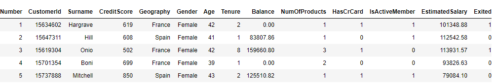
You can see the 14 columns in our dataset. Based on the first 13 columns, our task is to predict the value for the 14th column i.e. Exited. It is important to mention that the values for the first 13 columns are recorded 6 months before the value for the Exited column was obtained since the task is to predict customer churn after 6 months from the time when the customer information is recorded.
Exploratory Data Analysis
Let's perform some exploratory data analysis on our dataset. We'll first predict the ratio of the customer who actually left the bank after 6 months and will use a pie plot to visualize.
Let's first increase the default plot size for the graphs:
fig_size = plt.rcParams["figure.figsize"]
fig_size[0] = 10
fig_size[1] = 8
plt.rcParams["figure.figsize"] = fig_size
The following script draws the pie plot for the Exited column.
dataset.Exited.value_counts().plot(kind='pie', autopct='%1.0f%%', colors=['skyblue', 'orange'], explode=(0.05, 0.05))
Output:
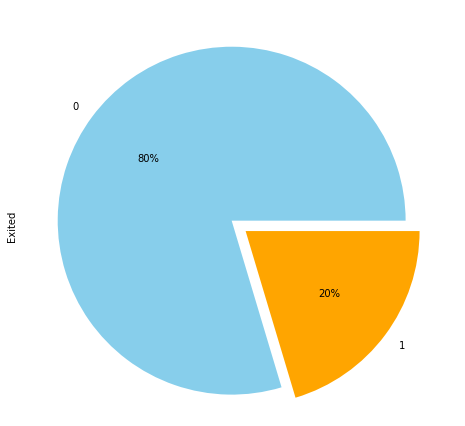
The output shows that in our dataset, 20% of the customers left the bank. Here 1 belongs to the case where the customer left the bank, where 0 refers to the scenario where a customer didn't leave the bank.
Let's plot the number of customers from all the geographical locations in the dataset:
sns.countplot(x='Geography', data=dataset)
Output:
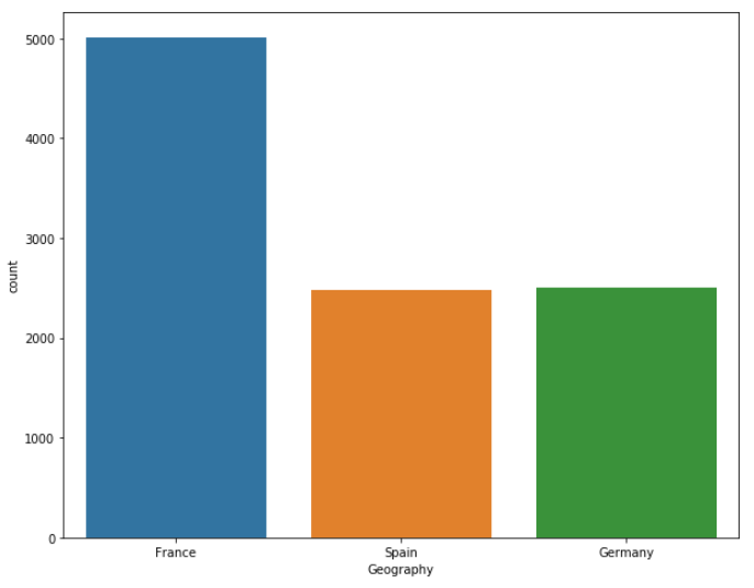
The output shows that almost half of the customers belong to France, while the ratio of customers belonging to Spain and Germany is 25% each.
Let's now plot number of customers from each unique geographical location along with customer churn information. We can use the countplot() function from the seaborn library to do so.
sns.countplot(x='Exited', hue='Geography', data=dataset)
Output:
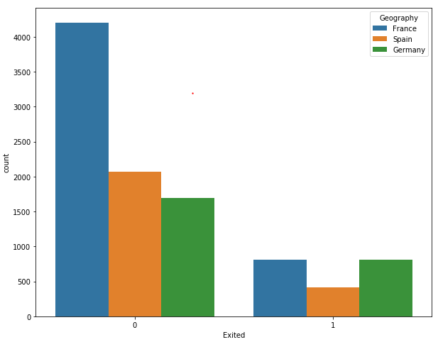
The output shows that though the overall number of French customers is twice that of the number of Spanish and German customers, the ratio of customers who left the bank is the same for French and German customers. Similarly, the overall number of German and Spanish customers is the same, but the number of German customers who left the bank is twice that of the Spanish customers, which shows that German customers are more likely to leave the bank after 6 months.
In this article, we will not visually plot the information related to the rest of the columns in our dataset, but if you want to do so, you check my article on how to perform exploratory data analysis with Python Seaborn Library.
Data Preprocessing
Before we train our PyTorch model, we need to preprocess our data. If you look at the dataset, you will see that it has two types of columns: Numerical and Categorical. The numerical columns contains numerical information. CreditScore, Balance, Age, etc. Similarly, Geography and Gender are categorical columns since they contain categorical information such as the locations and genders of the customers. There are a few columns that can be treated as numeric as well as categorical. For instance, the HasCrCard column can have 1 or 0 as its values. However, the HasCrCard columns contains information about whether or not a customer has credit card. It is advised that the column that can be treated as both categorical and numerical, are treated as categorical. However, it totally depends upon the domain knowledge of the dataset.
Let's again print all the columns in our dataset and find out which of the columns can be treated as numerical and which columns should be treated as categorical. The columns attribute of a dataframe prints all the column names:
dataset.columns
Output:
Index(['RowNumber', 'CustomerId', 'Surname', 'CreditScore', 'Geography',
       'Gender', 'Age', 'Tenure', 'Balance', 'NumOfProducts', 'HasCrCard',
       'IsActiveMember', 'EstimatedSalary', 'Exited'],
      dtype='object')
From the columns in our dataset, we will not use the RowNumber, CustomerId, and Surname columns since the values for these columns are totally random and have no relation with the output. For instance, a customer's surname has no impact on whether or not the customer will leave the bank. Among the rest of the columns, Geography, Gender, HasCrCard, and IsActiveMember columns can be treated as categorical columns. Let's create a list of these columns:
categorical_columns = ['Geography', 'Gender', 'HasCrCard', 'IsActiveMember']
All of the remaining columns except the Exited column can be treated as numerical columns.
numerical_columns = ['CreditScore', 'Age', 'Tenure', 'Balance', 'NumOfProducts', 'EstimatedSalary']
Finally, the output (the values from the Exited column) are stored in the outputs variable.
outputs = ['Exited']
We have created lists of categorical, numeric, and output columns. However, at the moment the type of the categorical columns is not categorical. You can check the type of all the columns in the dataset with the following script:
dataset.dtypes
Output:
RowNumber            int64
CustomerId           int64
Surname             object
CreditScore          int64
Geography           object
Gender              object
Age                  int64
Tenure               int64
Balance            float64
NumOfProducts        int64
HasCrCard            int64
IsActiveMember       int64
EstimatedSalary    float64
Exited               int64
dtype: object
You can see that the type for Geography and Gender columns is object and the type for HasCrCard and IsActive columns is int64. We need to convert the types for categorical columns to category. We can do so using the astype() function, as shown below:
for category in categorical_columns:
    dataset[category] = dataset[category].astype('category')
Now if you again plot the types for the columns in our dataset, you should see the following results:
dataset.dtypes
Output
RowNumber             int64
CustomerId            int64
Surname              object
CreditScore           int64
Geography          category
Gender             category
Age                   int64
Tenure                int64
Balance             float64
NumOfProducts         int64
HasCrCard          category
IsActiveMember     category
EstimatedSalary     float64
Exited                int64
dtype: object
Let's now see all the categories in the Geography column:
dataset['Geography'].cat.categories
Output:
Index(['France', 'Germany', 'Spain'], dtype='object')
When you change a column's data type to category, each category in the column is assigned a unique code. For instance, let's plot the first five rows of the Geography column and print the code values for the first five rows:
dataset['Geography'].head()
Output:
0    France
1     Spain
2    France
3    France
4     Spain
Name: Geography, dtype: category
Categories (3, object): [France, Germany, Spain]
The following script plots the codes for the values in the first five rows of the Geography column:
dataset['Geography'].head().cat.codes
Output:
0    0
1    2
2    0
3    0
4    2
dtype: int8
The output shows that France has been coded as 0, and Spain has been coded as 2.
The basic purpose of separating categorical columns from the numerical columns is that values in the numerical column can be directly fed into neural networks. However, the values for the categorical columns first have to be converted into numeric types. The coding of the values in the categorical column partially solves the task of numerical conversion of the categorical columns.
Since we will be using PyTorch for model training, we need to convert our categorical and numerical columns to tensors.
Let's first convert the categorical columns to tensors. In PyTorch, tensors can be created via the numpy arrays. We will first convert data in the four categorical columns into numpy arrays and then stack all the columns horizontally, as shown in the following script:
geo = dataset['Geography'].cat.codes.values
gen = dataset['Gender'].cat.codes.values
hcc = dataset['HasCrCard'].cat.codes.values
iam = dataset['IsActiveMember'].cat.codes.values

categorical_data = np.stack([geo, gen, hcc, iam], 1)

categorical_data[:10]
The above script prints the first five records from the categorical columns, stacked horizontally. The output is as follows:
Output:
array([[0, 0, 1, 1],
       [2, 0, 0, 1],
       [0, 0, 1, 0],
       [0, 0, 0, 0],
       [2, 0, 1, 1],
       [2, 1, 1, 0],
       [0, 1, 1, 1],
       [1, 0, 1, 0],
       [0, 1, 0, 1],
       [0, 1, 1, 1]], dtype=int8)
Now to create a tensor from the aforementioned numpy array, you can simply pass the array to the tensor class of the torch module. Remember, for the categorical columns the data type should be torch.int64.
categorical_data = torch.tensor(categorical_data, dtype=torch.int64)
categorical_data[:10]
Output:
tensor([[0, 0, 1, 1],
        [2, 0, 0, 1],
        [0, 0, 1, 0],
        [0, 0, 0, 0],
        [2, 0, 1, 1],
        [2, 1, 1, 0],
        [0, 1, 1, 1],
        [1, 0, 1, 0],
        [0, 1, 0, 1],
        [0, 1, 1, 1]])
In the output, you can see that the numpy array of categorical data has now been converted into a tensor object.
In the same way, we can convert our numerical columns to tensors:
numerical_data = np.stack([dataset[col].values for col in numerical_columns], 1)
numerical_data = torch.tensor(numerical_data, dtype=torch.float)
numerical_data[:5]
Output:
tensor([[6.1900e+02, 4.2000e+01, 2.0000e+00, 0.0000e+00, 1.0000e+00, 1.0135e+05],
        [6.0800e+02, 4.1000e+01, 1.0000e+00, 8.3808e+04, 1.0000e+00, 1.1254e+05],
        [5.0200e+02, 4.2000e+01, 8.0000e+00, 1.5966e+05, 3.0000e+00, 1.1393e+05],
        [6.9900e+02, 3.9000e+01, 1.0000e+00, 0.0000e+00, 2.0000e+00, 9.3827e+04],
        [8.5000e+02, 4.3000e+01, 2.0000e+00, 1.2551e+05, 1.0000e+00, 7.9084e+04]])
In the output, you can see the first five rows containing the values for the six numerical columns in our dataset.
The final step is to convert the output numpy array into a tensor object.
outputs = torch.tensor(dataset[outputs].values).flatten()
outputs[:5]
Output:
tensor([1, 0, 1, 0, 0])
Let now plot the shape of our categorial data, numerical data, and the corresponding output:
print(categorical_data.shape)
print(numerical_data.shape)
print(outputs.shape)
Output:
torch.Size([10000, 4])
torch.Size([10000, 6])
torch.Size([10000])
There is a one very important step before we can train our model. We converted our categorical columns to numerical where a unique value is represented by a single integer. For instance, in the Geography column, we saw that France is represented by 0 and Germany is represented by 1. We can use these values to train our model. However, a better way is to represent values in a categorical column is in the form of an N-dimensional vector, instead of a single integer. A vector is capable of capturing more information and can find relationships between different categorical values in a more appropriate way. Therefore, we will represent values in the categorical columns in the form of N-dimensional vectors. This process is called embedding.
We need to define the embedding size (vector dimensions) for all the categorical columns. There is no hard and fast rule regarding the number of dimensions. A good rule of thumb to define the embedding size for a column is to divide the number of unique values in the column by 2 (but not exceeding 50). For instance, for the Geography column, the number of unique values is 3. The corresponding embedding size for the Geography column will be 3/2 = 1.5 = 2 (round off).
The following script creates a tuple that contains the number of unique values and the dimension sizes for all the categorical columns:
categorical_column_sizes = [len(dataset[column].cat.categories) for column in categorical_columns]
categorical_embedding_sizes = [(col_size, min(50, (col_size+1)//2)) for col_size in categorical_column_sizes]
print(categorical_embedding_sizes)
Output:
[(3, 2), (2, 1), (2, 1), (2, 1)]
A supervised deep learning model, such as the one we are developing in this article, is trained using training data and the model performance is evaluated on the test dataset. Therefore, we need to divide our dataset into training and test sets as shown in the following script:
total_records = 10000
test_records = int(total_records * .2)

categorical_train_data = categorical_data[:total_records-test_records]
categorical_test_data = categorical_data[total_records-test_records:total_records]
numerical_train_data = numerical_data[:total_records-test_records]
numerical_test_data = numerical_data[total_records-test_records:total_records]
train_outputs = outputs[:total_records-test_records]
test_outputs = outputs[total_records-test_records:total_records]
We have 10 thousand records in our dataset, of which 80% records, i.e. 8000 records, will be used to train the model while the remaining 20% records will be used to evaluate the performance of our model. Notice, in the script above, the categorical and numerical data, as well as the outputs have been divided into the training and test sets.
To verify that we have correctly divided data into training and test sets, let's print the lengths of the training and test records:
print(len(categorical_train_data))
print(len(numerical_train_data))
print(len(train_outputs))

print(len(categorical_test_data))
print(len(numerical_test_data))
print(len(test_outputs))
Output:
8000
8000
8000
2000
2000
2000
Creating a Model for Prediction
We have divided the data into training and test sets, now is the time to define our model for training. To do so, we can define a class named Model, which will be used to train the model. Look at the following script:
class Model(nn.Module):

    def __init__(self, embedding_size, num_numerical_cols, output_size, layers, p=0.4):
        super().__init__()
        self.all_embeddings = nn.ModuleList([nn.Embedding(ni, nf) for ni, nf in embedding_size])
        self.embedding_dropout = nn.Dropout(p)
        self.batch_norm_num = nn.BatchNorm1d(num_numerical_cols)

        all_layers = []
        num_categorical_cols = sum((nf for ni, nf in embedding_size))
        input_size = num_categorical_cols + num_numerical_cols

        for i in layers:
            all_layers.append(nn.Linear(input_size, i))
            all_layers.append(nn.ReLU(inplace=True))
            all_layers.append(nn.BatchNorm1d(i))
            all_layers.append(nn.Dropout(p))
            input_size = i

        all_layers.append(nn.Linear(layers[-1], output_size))

        self.layers = nn.Sequential(*all_layers)

    def forward(self, x_categorical, x_numerical):
        embeddings = []
        for i,e in enumerate(self.all_embeddings):
            embeddings.append(e(x_categorical[:,i]))
        x = torch.cat(embeddings, 1)
        x = self.embedding_dropout(x)

        x_numerical = self.batch_norm_num(x_numerical)
        x = torch.cat([x, x_numerical], 1)
        x = self.layers(x)
        return x
If you have never worked with PyTorch before, the above code may look daunting, however I will try to break it down into for you.
In the first line, we declare a Model class that inherits from the Module class from PyTorch's nn module. In the constructor of the class (the __init__() method) the following parameters are passed:
embedding_size: Contains the embedding size for the categorical columnsnum_numerical_cols: Stores the total number of numerical columnsoutput_size: The size of the output layer or the number of possible outputs.layers: List which contains number of neurons for all the layers.p: Dropout with the default value of 0.5
Inside the constructor, a few variables are initialized. Firstly, the all_embeddings variable contains a list of ModuleList objects for all the categorical columns. The embedding_dropout stores the dropout value for all the layers. Finally, the batch_norm_num stores a list of BatchNorm1d objects for all the numerical columns.
Next, to find the size of the input layer, the number of categorical and numerical columns are added together and stored in the input_size variable. After that, a for loop iterates and the corresponding layers are added into the all_layers list. The layers added are:
Linear: Used to calculate the dot product between the inputs and weight matrixesReLu: Which is applied as an activation functionBatchNorm1d: Used to apply batch normalization to the numerical columnsDropout: Used to avoid overfitting
After the for loop, the output layer is appended to the list of layers. Since we want all of the layers in the neural networks to execute sequentially, the list of layers is passed to the nn.Sequential class.
Next, in the forward method, both the categorical and numerical columns are passed as inputs. The embedding of the categorical columns takes place in the following lines.
embeddings = []
for i, e in enumerate(self.all_embeddings):
    embeddings.append(e(x_categorical[:,i]))
x = torch.cat(embeddings, 1)
x = self.embedding_dropout(x)
The batch normalization of the numerical columns is applied with the following script:
x_numerical = self.batch_norm_num(x_numerical)
Finally, the embedded categorical columns x and the numeric columns x_numerical are concatenated together and passed to the sequential layers.
Training the Model
To train the model, first we have to create an object of the Model class that we defined in the last section.
model = Model(categorical_embedding_sizes, numerical_data.shape[1], 2, [200,100,50], p=0.4)
You can see that we pass the embedding size of the categorical columns, the number of numerical columns, the output size (2 in our case) and the neurons in the hidden layers. You can see that we have three hidden layers with 200, 100, and 50 neurons, respectively. You can choose any other size if you want.
Let's print our model and see how it looks:
print(model)
Output:
Model(
  (all_embeddings): ModuleList(
    (0): Embedding(3, 2)
    (1): Embedding(2, 1)
    (2): Embedding(2, 1)
    (3): Embedding(2, 1)
  )
  (embedding_dropout): Dropout(p=0.4)
  (batch_norm_num): BatchNorm1d(6, eps=1e-05, momentum=0.1, affine=True, track_running_stats=True)
  (layers): Sequential(
    (0): Linear(in_features=11, out_features=200, bias=True)
    (1): ReLU(inplace)
    (2): BatchNorm1d(200, eps=1e-05, momentum=0.1, affine=True, track_running_stats=True)
    (3): Dropout(p=0.4)
    (4): Linear(in_features=200, out_features=100, bias=True)
    (5): ReLU(inplace)
    (6): BatchNorm1d(100, eps=1e-05, momentum=0.1, affine=True, track_running_stats=True)
    (7): Dropout(p=0.4)
    (8): Linear(in_features=100, out_features=50, bias=True)
    (9): ReLU(inplace)
    (10): BatchNorm1d(50, eps=1e-05, momentum=0.1, affine=True, track_running_stats=True)
    (11): Dropout(p=0.4)
    (12): Linear(in_features=50, out_features=2, bias=True)
  )
)
You can see that in the first linear layer the value of the in_features variable is 11 since we have 6 numerical columns and the sum of embedding dimensions for the categorical columns is 5, hence 6+5 = 11. Similarly, in the last layer, the out_features has a value of 2 since we have only 2 possible outputs.
Before we can actually train our model, we need to define the loss function and the optimizer that will be used to train the model. Since, we are solving a classification problem, we will use the cross entropy loss. For the optimizer function, we will use the adam optimizer.
The following script defines the loss function and the optimizer:
loss_function = nn.CrossEntropyLoss()
optimizer = torch.optim.Adam(model.parameters(), lr=0.001)
Now we have everything that is needed to train the model. The following script trains the model:
epochs = 300
aggregated_losses = []

for i in range(epochs):
    i += 1
    y_pred = model(categorical_train_data, numerical_train_data)
    single_loss = loss_function(y_pred, train_outputs)
    aggregated_losses.append(single_loss)

    if i%25 == 1:
        print(f'epoch: {i:3} loss: {single_loss.item():10.8f}')

    optimizer.zero_grad()
    single_loss.backward()
    optimizer.step()

print(f'epoch: {i:3} loss: {single_loss.item():10.10f}')
The number of epochs is set to 300, which means that to train the model, the complete dataset will be used 300 times. A for loop executes for 300 times and during each iteration, the loss is calculated using the loss function. The loss during each iteration is appended to the aggregated_loss list. To update the weights, the backward() function of the single_loss object is called. Finally, the step() method of the optimizer function updates the gradient. The loss is printed after every 25 epochs.
The output of the script above is as follows:
epoch:   1 loss: 0.71847951
epoch:  26 loss: 0.57145703
epoch:  51 loss: 0.48110831
epoch:  76 loss: 0.42529839
epoch: 101 loss: 0.39972275
epoch: 126 loss: 0.37837571
epoch: 151 loss: 0.37133673
epoch: 176 loss: 0.36773482
epoch: 201 loss: 0.36305946
epoch: 226 loss: 0.36079505
epoch: 251 loss: 0.35350436
epoch: 276 loss: 0.35540250
epoch: 300 loss: 0.3465710580
The following script plots the losses against epochs:
plt.plot(range(epochs), aggregated_losses)
plt.ylabel('Loss')
plt.xlabel('epoch');
Output:
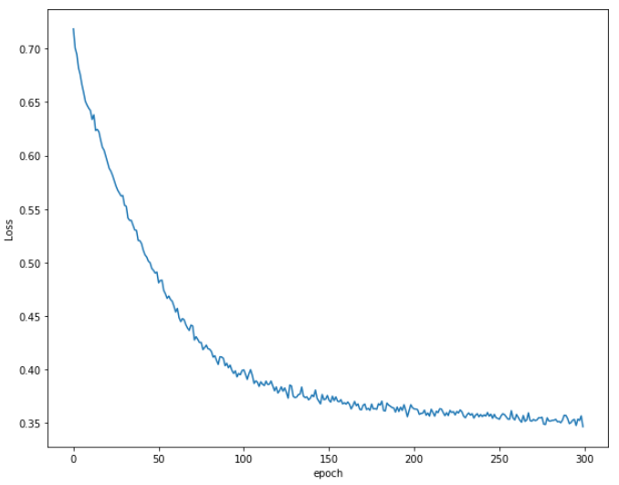
The output shows that initially the loss decreases rapidly. After around the 250th epoch, there is a very little decrease in the loss.
Making Predictions
The last step is to make predictions on the test data. To do so, we simply need to pass the categorical_test_data and numerical_test_data to the model class. The values returned can then be compared with the actual test output values. The following script makes predictions on the test class and prints the cross entropy loss for the test data.
with torch.no_grad():
    y_val = model(categorical_test_data, numerical_test_data)
    loss = loss_function(y_val, test_outputs)
print(f'Loss: {loss:.8f}')
Output:
Loss: 0.36855841
The loss on the test set is 0.3685, which is slightly more than 0.3465 achieved on the training set which shows that our model is slightly overfitting.
It is important to note that since we specified that our output layer will contain 2 neurons, each prediction will contain 2 values. For instance, the first 5 predicted values look like this:
print(y_val[:5])
Output:
tensor([[ 1.2045, -1.3857],
        [ 1.3911, -1.5957],
        [ 1.2781, -1.3598],
        [ 0.6261, -0.5429],
        [ 2.5430, -1.9991]])
The idea behind such predictions is that if the actual output is 0, the value at the index 0 should be higher than the value at index 1, and vice versa. We can retrieve the index of the largest value in the list with the following script:
y_val = np.argmax(y_val, axis=1)
Output:
Let's now again print the first five values for the y_val list:
print(y_val[:5])
Output:
tensor([0, 0, 0, 0, 0])
Since in the list of originally predicted outputs, for the first five records, the the values at zero indexes are greater than the values at first indexes, we can see 0 in the first five rows of the processed outputs.
Finally, we can use the confusion_matrix, accuracy_score, and classification_report classes from the sklearn.metrics module to find the accuracy, precision, and recall values for the test set, along with the confusion matrix.
from sklearn.metrics import classification_report, confusion_matrix, accuracy_score

print(confusion_matrix(test_outputs,y_val))
print(classification_report(test_outputs,y_val))
print(accuracy_score(test_outputs, y_val))
Output:
[[1527   83]
 [ 224  166]]
              precision    recall  f1-score   support

           0       0.87      0.95      0.91      1610
           1       0.67      0.43      0.52       390

   micro avg       0.85      0.85      0.85      2000
   macro avg       0.77      0.69      0.71      2000
weighted avg       0.83      0.85      0.83      2000

0.8465
The output shows that our model achieves an accuracy of 84.65% which is pretty impressive given the fact that we randomly selected all the parameters for our neural network model. I would suggest that you try to change the model parameters i.e. train/test splits, number and size of hidden layers, etc. to see if you can get better results.
Conclusion
PyTorch is a commonly used deep learning library developed by Facebook which can be used for a variety of tasks such as classification, regression, and clustering. This article explains how to use PyTorch library for the classification of tabular data.
↧
Podcast.__init__: Illustrating The Landscape And Applications Of Deep Learning
Deep learning is a phrase that is used more often as it continues to transform the standard approach to artificial intelligence and machine learning projects. Despite its ubiquity, it is often difficult to get a firm understanding of how it works and how it can be applied to a particular problem. In this episode Jon Krohn, author of Deep Learning Illustrated, shares the general concepts and useful applications of this technique, as well as sharing some of his practical experience in using it for his work. This is definitely a helpful episode for getting a better comprehension of the field of deep learning and when to reach for it in your own projects.![]()
Summary
Deep learning is a phrase that is used more often as it continues to transform the standard approach to artificial intelligence and machine learning projects. Despite its ubiquity, it is often difficult to get a firm understanding of how it works and how it can be applied to a particular problem. In this episode Jon Krohn, author of Deep Learning Illustrated, shares the general concepts and useful applications of this technique, as well as sharing some of his practical experience in using it for his work. This is definitely a helpful episode for getting a better comprehension of the field of deep learning and when to reach for it in your own projects.
Announcements
- Hello and welcome to Podcast.__init__, the podcast about Python and the people who make it great.
- When you’re ready to launch your next app or want to try a project you hear about on the show, you’ll need somewhere to deploy it, so take a look at our friends over at Linode. With 200 Gbit/s private networking, scalable shared block storage, node balancers, and a 40 Gbit/s public network, all controlled by a brand new API you’ve got everything you need to scale up. And for your tasks that need fast computation, such as training machine learning models, they just launched dedicated CPU instances. Go to pythonpodcast.com/linode to get a $20 credit and launch a new server in under a minute. And don’t forget to thank them for their continued support of this show!
- You listen to this show to learn and stay up to date with the ways that Python is being used, including the latest in machine learning and data analysis. For even more opportunities to meet, listen, and learn from your peers you don’t want to miss out on this year’s conference season. We have partnered with organizations such as O’Reilly Media, Dataversity, Corinium Global Intelligence, Alluxio, and Data Council. Upcoming events include the combined events of the Data Architecture Summit and Graphorum, the Data Orchestration Summit, and Data Council in NYC. Go to pythonpodcast.com/conferences to learn more about these and other events, and take advantage of our partner discounts to save money when you register today.
- Your host as usual is Tobias Macey and today I’m interviewing Jon Krohn about his recent book, deep learning illustrated
Interview
- Introductions
- How did you get introduced to Python?
- Can you start by giving a brief description of what we’re talking about when we say deep learning and how you got involved with the field?
- How does your background in neuroscience factor into your work on designing and building deep learning models?
- What are some of the ways that you leverage deep learning techniques in your work?
- What was your motivation for writing a book on the subject?
- How did the idea of including illustrations come about and what benefit do they provide as compared to other books on this topic?
- While planning the contents of the book what was your thought process for determining the appropriate level of depth to cover?
- How would you characterize the target audience and what level of familiarity and proficiency in employing deep learning do you wish them to have at the end of the book?
- How did you determine what to include and what to leave out of the book?
- The sequencing of the book follows a useful progression from general background to specific uses and problem domains. What were some of the biggest challenges in determining which domains to highlight and how deep in each subtopic to go?
- Because of the continually evolving nature of the field of deep learning and the associated tools, how have you guarded against obsolescence in the content and structure of the book?
- Which libraries did you focus on for your examples and what was your selection process?
- Now that it is published, is there anything that you would have done differently?
- Which libraries did you focus on for your examples and what was your selection process?
- One of the critiques of deep learning is that the models are generally single purpose. How much flexibility and code reuse is possible when trying to repurpose one model pipeline for a slightly different dataset or use case?
- I understand that deployment and maintenance of models in production environments is also difficult. What has been your experience in that regard, and what recommendations do you have for practitioners to reduce their complexity?
- What is involved in actually creating and using a deep learning model?
- Can you go over the different types of neurons and the decision making that is required when selecting the network topology?
- In terms of the actual development process, what are some useful practices for organizing the code and data that goes into a model, given the need for iterative experimentation to achieve desired levels of accuracy?
- What is your personal workflow when building and testing a new model for a new use case?
- What are some of the limitations of deep learning and cases where you would recommend against using it?
- What are you most excited for in the field of deep learning and its applications?
- What are you most concerned by?
- Do you have any parting words or closing advice for listeners and potential readers?
Keep In Touch
- Website
- @jonkrohnlearns on Twitter
- jonkrohn on GitHub
Picks
- Tobias
- Jon
- Data Elixir Newsletter
Closing Announcements
- Thank you for listening! Don’t forget to check out our other show, the Data Engineering Podcast for the latest on modern data management.
- Visit the site to subscribe to the show, sign up for the mailing list, and read the show notes.
- If you’ve learned something or tried out a project from the show then tell us about it! Email hosts@podcastinit.com) with your story.
- To help other people find the show please leave a review on iTunes and tell your friends and co-workers
- Join the community in the new Zulip chat workspace at pythonpodcast.com/chat
Links
- Untapt
- Deep Learning Illustrated
- Pearson
- Columbia University
- New York City Data Science Academy
- NIH (National Institutes of Health)
- Oxford Uniersity
- Matlab
- R Language
- Neuroscience
- Artificial Neural Network
- Deep Learning
- Natural Language Processing
- Computer Vision
- Generative Adversarial Networks
- Deep Learning by Ian Goodfellow, et al.
- Hands On Machine Learning by Aurélien Géron
- O’Reilly Online Learning
- Transfer Learning
- Keras
- Tensorflow
- PyTorch
- Gary Marcus
- Judea Pearl
- Artificial General Intelligence
- Explainable AI
- Yuval Noah Harrari
- Wait But Why?
The intro and outro music is from Requiem for a Fish The Freak Fandango Orchestra / CC BY-SA
↧
IslandT: Python array list’s count method
In this example, we will use the count method from the Python array list to decide which phrase to return from a function that will accept an array list consists of good and bad ideas.
In the below example, you need to decide which phrase to return from the array list which consists of good ideas ‘good’ and bad ideas ‘bad’. If there are one or two good ideas, return ‘Publish!’, if there are more than 2 return ‘I smell a series!’. If there are no good ideas, as is often the case, return ‘Fail!’.
def well(x):

    if x.count('good') > 2:

        return 'I smell a series!'

    elif x.count('good') > 0:

        return 'Publish!'

    else:

        return 'Fail!'
Write down your own python answer in below comment box.
If you like this post do share the post on any social media site to help this site to grow, thank you.
↧
Tryton News: Tryton Spanish Days 2019: In Alicante on the 27th & 28th of November
@pokoli wrote:
The Tryton Foundation is happy to announce the venue and date of the next Tryton Spanish Days.
The event will take place in the sunny city of Alicante on the 27th and 28th of November at the Auditorio Puerta Ferrisa at Calle Jorge Juan, 21, 03002 Alicante
Several Tryton experts will talk about open source and digital transformation . We will discuss some challenges related to mobility, Internet of Things and Integrations with other systems. Several companies will share their experience using open source software like Tryton. More details will come when we publish the schedule.
Register (in Spanish).

Posts: 1
Participants: 1
↧
↧
S. Lott: State Change and NoSQL Databases
Let's take another look at F. L. Stevens spreadsheet with agencies and agents. It's -- of course -- an unholy mess. Why? It's difficult to handle state change and deduplication.
Let's look at state changes.
The author needs URL's and names and a list of genres the agent is interested in. This is more-or-less static data. It changes rarely. What changes more often is an agent being closed or open to queries.
Another state change is the query itself. Once the email has been sent, the agent (and their agency) should not be bothered again for at least sixty days. After an explicit rejection, there's little point in making any contact with the agent; they're effectively out of the market for a given manuscript.
There are some other stateful rules, we don't need all the details to see the potential complexities here.
A spreadsheet presents a particularly odious non-solution to the problem of state and state change. There's a good and a bad. Mostly bad.
We can try to spread history down the rows of a column. Wow this is bad. We can try to use the hierarchy features to make history a bunch of folded-up details underneath a heading row. This is microscopically better, but still difficult to manage with all the unfolding and folding required to change state after a rejection.
We can blow up a single cell to have non-atomic data -- all of the history with events and dates in a long, ";" delimited list.
There's no good way to represent this in a spreadsheet.
The rigidity of the SQL schema is a barrier here. We're dealing with some sloppy data handling practices in the legacy spreadsheet. We don't want to have to tweak the SQL each time we find some new subtlety that's poorly represented in the spreadsheet data.
We're also handling a number of data sources, each with a unique schema. We need a way to unify these flexibly, so we can fold in additional data sources, once the broken spreadsheet is behind us.
(There are a yet more problems with the relational model in general, those are material for a separate blog post. For now, the rigidity and complexity are a big enough pair of problems.)
We have an Agency as the primary document., Within an Agency, there are a number of individual Agents. Within each agent is a series of Events. Some Agents aren't even interested in the genre F. L. Stevens writes, so they're closed. Some Agents are temporarily closed. The rest are open.
The author can get a list of open agents, following a number of rules, including waiting after the last contact, and avoiding working with multiple agents within a single agency. After sending query letters, the event history gets an entry, and those agents are in another state, query pending.
One common complaint I hear about a document store is the "cost" of updating a large-ish document. The implicit assumption seems to be that an update operation can't locate the relevant sub-document, and can't make incremental changes. Having worked with both SQL and NoSQL, this "cost of document update" seems to be unmeasurably small.
Another cluster command question hovers around locking and concurrency. Most of them nonsensical because they come from the world of fragmented data in a SQL database. When the relevant object (i.e. Agency) is spread over a lot of rows of several tables, locking is essential. When the relevant object is a single document, locks aren't as important. If two people are updating the same document at the same time, that's a document design issue, or a control issue in the application.
Finally, there are questions about "update anomalies." This is a sensible question. In the relational world, we often have shared "lookup" data. A single change to a lookup row will have a ripple effect to all rows using the lookup row's foreign key.
Think of changing zip code 12345 from Schenectady, NY to Scotia, NY. Everyone sharing the foreign key reference via the zip code has been moved with a single update. Except, of course, nothing is visible until a query reconstructs the desired document from the fragmented pieces.
We've traded a rare sweeping updated across many documents for a sweeping, complex join operating to build the relevant document from the normalized pieces. Queries are expensive, complex, and often wrong. They're so painful, we use ORM's to mask the queries and give us the documents we wanted all along.
We have three classes here. Agency is the parent document. Each Agency contains one or more Agent instances. Each Agent contains one or more Events.
When we fetch an agent's data, we fetch the entire agency, since the "business" rules preclude querying more than one agent in an agency. The queries involve a nuanced state change: a rejection by one agent, opens another in the same agency. Rather than do some additional SQL queries to locate the parent and other children of the parent, just read the whole thing at once.
In later posts, we'll look at deduplication and some other processing. But this seems to be all the schema we'll ever need. The type hints provided mypy some evidence of what we intend to do with these documents.
Let's look at state changes.
The author needs URL's and names and a list of genres the agent is interested in. This is more-or-less static data. It changes rarely. What changes more often is an agent being closed or open to queries.
Another state change is the query itself. Once the email has been sent, the agent (and their agency) should not be bothered again for at least sixty days. After an explicit rejection, there's little point in making any contact with the agent; they're effectively out of the market for a given manuscript.
There are some other stateful rules, we don't need all the details to see the potential complexities here.
A spreadsheet presents a particularly odious non-solution to the problem of state and state change. There's a good and a bad. Mostly bad.
- On the good side, you can edit a single cell, changing the state. You can define a drop-down list of states, or radio buttons with alternative states.
- The be bad side, you're often limited to editing a single cell when you want to change the state. You want to have dates filled in automatically on state change. You want history of state changes. Excel hackers try to write macros to automate filling in the date. History, however... History is a problem.
We can try to spread history down the rows of a column. Wow this is bad. We can try to use the hierarchy features to make history a bunch of folded-up details underneath a heading row. This is microscopically better, but still difficult to manage with all the unfolding and folding required to change state after a rejection.
We can blow up a single cell to have non-atomic data -- all of the history with events and dates in a long, ";" delimited list.
There's no good way to represent this in a spreadsheet.
What to do?
The relational database people love the master-detail relationship. Agency has Agent. Agent has History. The history is a bunch of rows in the history table, with a foreign key relationship with the agent.The rigidity of the SQL schema is a barrier here. We're dealing with some sloppy data handling practices in the legacy spreadsheet. We don't want to have to tweak the SQL each time we find some new subtlety that's poorly represented in the spreadsheet data.
We're also handling a number of data sources, each with a unique schema. We need a way to unify these flexibly, so we can fold in additional data sources, once the broken spreadsheet is behind us.
(There are a yet more problems with the relational model in general, those are material for a separate blog post. For now, the rigidity and complexity are a big enough pair of problems.)
SQL is Out. What Else?
A document store is pretty nice for this. The rest of this section is an indictment of SQL. Feel free to skip it. It's widely known, and well supported elsewhere.We have an Agency as the primary document., Within an Agency, there are a number of individual Agents. Within each agent is a series of Events. Some Agents aren't even interested in the genre F. L. Stevens writes, so they're closed. Some Agents are temporarily closed. The rest are open.
The author can get a list of open agents, following a number of rules, including waiting after the last contact, and avoiding working with multiple agents within a single agency. After sending query letters, the event history gets an entry, and those agents are in another state, query pending.
One common complaint I hear about a document store is the "cost" of updating a large-ish document. The implicit assumption seems to be that an update operation can't locate the relevant sub-document, and can't make incremental changes. Having worked with both SQL and NoSQL, this "cost of document update" seems to be unmeasurably small.
Another cluster command question hovers around locking and concurrency. Most of them nonsensical because they come from the world of fragmented data in a SQL database. When the relevant object (i.e. Agency) is spread over a lot of rows of several tables, locking is essential. When the relevant object is a single document, locks aren't as important. If two people are updating the same document at the same time, that's a document design issue, or a control issue in the application.
Finally, there are questions about "update anomalies." This is a sensible question. In the relational world, we often have shared "lookup" data. A single change to a lookup row will have a ripple effect to all rows using the lookup row's foreign key.
Think of changing zip code 12345 from Schenectady, NY to Scotia, NY. Everyone sharing the foreign key reference via the zip code has been moved with a single update. Except, of course, nothing is visible until a query reconstructs the desired document from the fragmented pieces.
We've traded a rare sweeping updated across many documents for a sweeping, complex join operating to build the relevant document from the normalized pieces. Queries are expensive, complex, and often wrong. They're so painful, we use ORM's to mask the queries and give us the documents we wanted all along.
What's It Look Like?
This:@dataclass
class Agency:
"""A collection of individual agents."""
name : str
url : Optional[str] = field(default=None)
agents : Dict[str, 'Agent'] = field(init=False, default_factory=dict)
@dataclass
class Agent:
"""An Agent with a sequence of events: actions and state changes."""
name : str
url : str
email : str
fiction_genres : List[str]
query_details : str = field(default_factory=str)
events : List['Event'] = field(init=False, default_factory=list)
@dataclass
class Event:
"""An action or state change.
status = 'open', 'closed', 'query sent', 'query outcome', 'closed until', etc.
Depending on the status, there may be additional details.
For 'query sent', there's 'date'.
For 'query outcome', there's 'outcome' and an optional 'date'.
for 'closed until', there's 'reason' and an optional 'date'.
"""
status : str
date : Optional[datetime.date] = field(default=None)
outcome : Optional[str] = field(default=None)
reason : Optional[str] = field(default=None)
def __repr__(self):
return f"{self.status} {self.date} {self.outcome} {self.reason}"
We have three classes here. Agency is the parent document. Each Agency contains one or more Agent instances. Each Agent contains one or more Events.
When we fetch an agent's data, we fetch the entire agency, since the "business" rules preclude querying more than one agent in an agency. The queries involve a nuanced state change: a rejection by one agent, opens another in the same agency. Rather than do some additional SQL queries to locate the parent and other children of the parent, just read the whole thing at once.
In later posts, we'll look at deduplication and some other processing. But this seems to be all the schema we'll ever need. The type hints provided mypy some evidence of what we intend to do with these documents.
↧
NumFOCUS: NumFOCUS and Tidelift partner to support essential community-led open source data science and scientific computing projects
↧
Django Weblog: Nominations for 2019 Malcolm Tredinnick Memorial Prize
It is that time of year again when we recognize someone from our community in memory of our friend Malcolm.
Malcolm was an early core contributor to Django and had both a huge influence and large impact on Django as we know it today. Besides being knowledgeable he was also especially friendly to new users and contributors. He exemplified what it means to be an amazing Open Source contributor. We still miss him.
The DSF Prize page summarizes the prize nicely:
The Malcolm Tredinnick Memorial Prize is a monetary prize, awarded annually, to the person who best exemplifies the spirit of Malcolm’s work - someone who welcomes, supports and nurtures newcomers; freely gives feedback and assistance to others, and helps to grow the community. The hope is that the recipient of the award will use the award stipend as a contribution to travel to a community event -- a DjangoCon, a PyCon, a sprint -- and continue in Malcolm’s footsteps.
We will take nominations until Friday, November 8th AoE and will announce the winner soon after. Please make your nominations using this google form.
If you have any questions please reach out to the DSF Board at foundation@djangoproject.com.
↧
Real Python: Python Plotting With Matplotlib
A picture is worth a thousand words, and with Python’s matplotlib library, it fortunately takes far less than a thousand words of code to create a production-quality graphic.
However, matplotlib is also a massive library, and getting a plot to look just right is often achieved through trial and error. Using one-liners to generate basic plots in matplotlib is relatively simple, but skillfully commanding the remaining 98% of the library can be daunting.
In this beginner-friendly course, you’ll learn about plotting in Python with matplotlib by looking at the theory and following along with practical examples. While learning by example can be tremendously insightful, it helps to have even just a surface-level understanding of the library’s inner workings and layout as well.
By the end of this course, you’ll:
- Know the differences between PyLab and Pyplot
- Grasp the key concepts in the design of
matplotlib - Understand
plt.subplots() - Visualize arrays with
matplotlib - Plot by combining
pandasandmatplotlib
This course assumes you know a tiny bit of NumPy. You’ll mainly use the numpy.random module to generate “toy” data, drawing samples from different statistical distributions. If you don’t already have matplotlib installed, see the documentation for a walkthrough before proceeding.
[ Improve Your Python With 🐍 Python Tricks 💌 – Get a short & sweet Python Trick delivered to your inbox every couple of days. >> Click here to learn more and see examples ]
↧
↧
PyCon: Startup Row PyCon US 2020 Applications are Open!
Another year, another PyCon US, another opportunity for early-stage startups to show off how they use Python on Startup Row. Every PyCon since 2011, the Python Software Foundation has given qualifying early-stage startups complimentary access to the best of what PyCon has to offer.
If you’re one of those “apply first and read things later” sorts of folks, first create an account and then click here to get started! It should only take a few minutes to register and confirm your user account, and then to fill out the form. Applications are due by January 17, 2020!
Startup Row at PyCon US is the PSF’s way of giving back to the startup ecosystem, and your opportunity to connect with the thousands of developers, data scientists, researchers, students, and enthusiasts who come to PyCon US each year.
Does your startup qualify? Here are the criteria:
Other Startup Row alumni companies include Textio (SR’16), X.ai (SR’15), Nylas (SR’14), Plotly (SR’13), Pandas developer Lambda Foundry (SR’12), and DotCloud (SR’11) which later pivoted to become Docker.
PyCon Startup Row companies have collectively raised nearly $1 billion in venture capital funding and have been acquired by the likes of Amazon, Splunk, Rackspace, and Baidu, among others.
It’s a competitive process. We review all applications that come in, and organizers are happy to answer any questions you might have about the PyCon experience or your application.
Apply by January 17, 2020! Remember that you need to create an account on the PyCon US website first, before applying.
Blog written by Jason D. Rowley, Chair, Startup Row Committee
If you’re one of those “apply first and read things later” sorts of folks, first create an account and then click here to get started! It should only take a few minutes to register and confirm your user account, and then to fill out the form. Applications are due by January 17, 2020!
Startup Row at PyCon US is the PSF’s way of giving back to the startup ecosystem, and your opportunity to connect with the thousands of developers, data scientists, researchers, students, and enthusiasts who come to PyCon US each year.
Does your startup qualify? Here are the criteria:
- You use Python somewhere in your tech or business stack (open source, proprietary, data science, machine learning, orchestration, marketing automation… it all counts)
- Your startup is 2.5 years old, or less, at time of applying (if you had a major pivot or delayed product launch, measure from there)
- You have 15 or fewer full-time employees, including founders, at the time of applying
- You or your company will fund travel and accommodation to PyCon US in Pittsburgh, PA
- You have not previously presented on Startup Row at PyCon (if you applied before but didn’t make it, you’re encouraged to apply again!)
- Two conference passes (you’re welcome to stay for the post-conference sprints too)
- Booth space on Startup Row in the Expo Hall for April 17-18, 2020
- Access to the PyCon Jobs Fair on April 19, 2020
- A group breakfast
- Eternal glory
Other Startup Row alumni companies include Textio (SR’16), X.ai (SR’15), Nylas (SR’14), Plotly (SR’13), Pandas developer Lambda Foundry (SR’12), and DotCloud (SR’11) which later pivoted to become Docker.
PyCon Startup Row companies have collectively raised nearly $1 billion in venture capital funding and have been acquired by the likes of Amazon, Splunk, Rackspace, and Baidu, among others.
It’s a competitive process. We review all applications that come in, and organizers are happy to answer any questions you might have about the PyCon experience or your application.
Apply by January 17, 2020! Remember that you need to create an account on the PyCon US website first, before applying.
Blog written by Jason D. Rowley, Chair, Startup Row Committee
↧
PyCharm: Webinar: “Visual SQL Development with PyCharm” with Maxim Sobolevskiy
We talk about visual debugging, visual testing, etc. But… visual databasing? Indeed, PyCharm embeds DataGrip, our IDE for SQL development.
In this webinar Maxim Sobolevskiy, the DataGrip Product Marketing Manager, gives us a whirlwind tour of one of the most exciting parts of PyCharm that most of us don’t know enough about. DataGrip is not just magic, it’s wildly useful and productive magic. Maxim will show us how to put it to work.
- Wednesday, November 6th
- 6:00 PM – 7:00 PM CET (12:00 PM – 1:00 PM EST)
- Register here
- Aimed at SQL developers

Speaking To You
Maxim Sobolevskiy was an SQL developer for 10 years. Since the Summer of 2015 he does marketing for the JetBrains SQL IDE called DataGrip.
↧
PyCoder’s Weekly: Issue #391 (Oct. 22, 2019)
#391 – OCTOBER 22, 2019
View in Browser »
Arduino Microcontrollers + Python: How to Get Started
Discover how to use Arduino microcontrollers with Python to develop your own electronic projects. You’ll learn how to set up circuits and write applications with the Firmata protocol. You’ll control Arduino inputs and outputs and integrate the board with higher-level apps.
REAL PYTHON
Let’s Write an LLVM Specializer for Python
“We’re going to build a single module Numba-like compiler for Python. It won’t be nearly as featureful or complete, but should demonstrate how you can go about building your own little LLVM specializer for a subset of Python or your own custom DSL expression compiler; and integrating it with the standard NumPy/SciPy stack for whatever scientific computing domain you work.”
STEPHEN DIEHL
SQL, Python, and R. All in One Platform. Free Forever.
Mode Studio combines a SQL editor, Python & R notebooks, and visualization builder in one platform. Connect your data warehouse and analyze with your preferred language. Make custom viz (D3.js, HTML/CSS) or use out-of-the-box charts →
MODE ANALYTICSsponsor
Python 2.7.17 Released
Python 2.7.17 is a bug fix release in the Python 2.7.x series. It is expected to be the penultimate release for Python 2.7. Full changelog here.
PYTHON.ORG
Python Code Complexity Waterfall
What can be done to prevent your Python code from getting too complex? A good linter setup does much more than finding missing commas and bad quotes. A good linter allows you to rely on it with architecture decisions and help you with the refactoring process.
NIKITA SOBOLEV
Reimplementing a Solaris Command in Python Gained 17x Performance Improvement From C
“As a result of fixing a memory allocation issue in the /usr/bin/listusers command, that had caused issues when it was converted to 64 bit, I decided to investigate if this ancient C code could be improved by conversion to Python.”
DARREN MOFFAT
The Simple Essence of the Y Combinator (Explained in Python)
“The Y combinator is a central concept in lambda calculus, which is the formal foundation of functional languages. Y allows one to define recursive functions without using self-referential definitions.”
LIONEL PARREAUX
Python at Scale: Strict Modules
The Instagram engineering team is experimenting with a technique for writing Python modules that are side-effect-free on import to reduce server startup time and unexpected global state changes.
CARL MEYER
Python Attribute Access and the Descriptor Protocol
A deep dive into Python attribute access and the descriptor protocol. What exactly happens when we say foo.bar?
AMIR RACHUM
Discussions
Python Jobs
Full Stack Developer (Toronto, ON, Canada)
Backend Developer (Kfar Saba, Israel)
Articles & Tutorials
time.sleep(): How to Add Time Delays to Your Code
Learn how to add time delays to your Python programs. You’ll use decorators and the built-in time module to add Python sleep() calls to your code. Then, you’ll discover how time delays work with threads, asynchronous functions, and graphical user interfaces.
REAL PYTHON
7 Common Mistakes That Django Developers Make
“Django is powerful web framework, but with power comes responsibility. In this article, we will cover common mistakes that are even seasoned Django developers make, yet most successful Django projects need to deal with these sooner or later.”
TOMASZ BĄK• Shared by Tomasz Bąk
Python Developers Are in Demand on Vettery
Vettery is an online hiring marketplace that’s changing the way people hire and get hired. Ready for a bold career move? Make a free profile, name your salary, and connect with hiring managers from top employers today →
VETTERYsponsor
Beyond cProfile: Sampling Profilers and Logging for Performance Optimization
“Your Python program is too slow. Maybe your web application can’t keep up, or certain queries are taking a long time. Maybe you have a batch program that takes hours or even days to run. How do you speed it up?”
ITAMAR TURNER-TRAURING
Flying High With Vaex: Analysis of Over 30 Years of Flight Data in Python
“Using the Python DataFrame library Vaex, I present the analysis of nearly 200 million flights made by U.S. carriers. Vaex uses fast out-of-core algorithms, making memory issues a thing of the past.”
JOVAN VELJANOSKI
Converting HTML to a Jupyter Notebook
“Learn how to scrape code from a webpage and save it as a Jupyter notebook. In this post, we’ll use Beautifulsoup4, urllib, and json, to save HTML to .ipynb.”
ERIK MARSJA
Python Plotting With Matplotlib
Want to make beautiful plots? Learn about plotting in Python with matplotlib by looking at the theory and following along with practical examples.
REAL PYTHONvideo
Keras vs tf.keras: What’s the Difference in TensorFlow 2.0?
In this tutorial you’ll discover the difference between Keras and tf.keras. You’ll also learn what’s new in TensorFlow 2.0.
ADRIAN ROSEBROCK
Designing CI/CD Systems: Painless Status Reporting in GitHub Pull Requests
How to report status from Docker containers in an automated CI/CD system into GitHub pull requests using Python.
CRISTIAN MEDINA• Shared by Cristian Medina
Pylint: Making Your Python Code Consistent
How to configure the Pylint code linter to avoid arguing about code complexity.
MOSHE ZADKA
Python 2 EOL: Are You Prepared? Take ActiveState’s Survey for a Chance to Win a Drone
Python 2 End of Life is coming soon. Take ActiveState’s 5-minute survey to let them know how you’re preparing for the change. You’ll get the final results, plus the chance to win a camera drone.
ACTIVESTATEsponsor
Projects & Code
ssis_validator: Validate SQL Server Integration Services (SSIS) Packages
GITHUB.COM/MAHDI-HOSSEINI• Shared by Mike
Events
Python Brasil 2019
October 23 to October 29, 2019
PYTHONBRASIL.ORG.BR
PythOnRio Meetup
October 26, 2019
PYTHON.ORG.BR
PyCon Sweden 2019
October 31 to November 2, 2019
PYCON.SE
Happy Pythoning!
This was PyCoder’s Weekly Issue #391.
View in Browser »
[ Subscribe to 🐍 PyCoder’s Weekly 💌 – Get the best Python news, articles, and tutorials delivered to your inbox once a week >> Click here to learn more ]
↧