Python & SharePoint might seem like a odd combination, but you can get useful information out of SharePoint by using a simple Python script.
↧
Codementor: How I access Microsoft SharePoint in my Python scripts
↧
Robin Wilson: Easily hiding items from the legend in matplotlib
When producing some graphs for a client recently, I wanted to hide some labels from a legend in matplotlib. I started investigating complex arguments to the plt.legend function, but it turned out that there was a really simple way to do it…
If you start your label for a plot item with an underscore (_) then that item will be hidden from the legend.
For example:
plt.plot(np.random.rand(20), label='Random 1')
plt.plot(np.random.rand(20), label='Random 2')
plt.plot(np.random.rand(20), label='_Hidden label')
plt.legend()
produces a plot like this:
You can see that the third line is hidden from the legend – just because we started its label with an underscore.
I found this particularly useful when I wanted to plot a load of lines in the same colour to show all the data for something, and then highlight a few lines that meant specific things. For example:
for i in range(20):
    plt.plot(np.random.rand(20), label='_Hidden', color='gray', alpha=0.3)
plt.plot(np.random.rand(20), label='Important Line 1')
plt.plot(np.random.rand(20), label='Important Line 2')
plt.legend()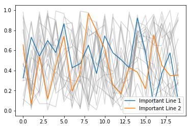
My next step was to do this when plotting from pandas. In this case I had a dataframe that had a column for each line I wanted to plot in the ‘background’, and then a separate dataframe with each of the ‘special’ lines to highlight.
This code will create a couple of example dataframes:
df = pd.DataFrame()

for i in range(20):
    df[f'Data{i}'] = np.random.rand(20)

special = pd.Series(data=np.random.rand(20))
Plotting this produces a legend with all the individual lines showing:
df.plot(color='gray', alpha=0.3)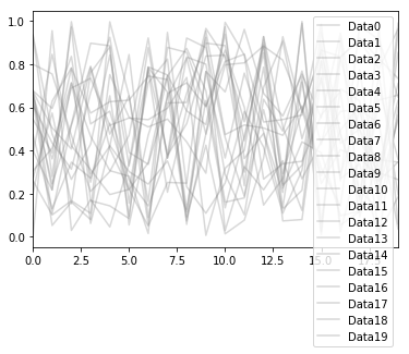
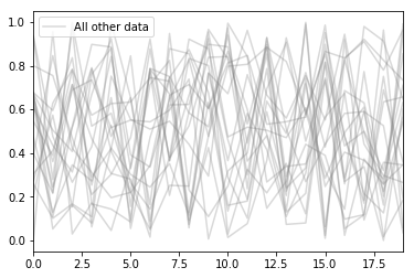
However, just by changing the column names to start with an underscore you can hide all the entries in the legend. In this example, I actually set one of the columns to a name without an underscore, so that column can be used as a label to represent all of these lines:
cols = ["_" + col for col in df.columns]
cols[0] = 'All other data'
df.columns = cols
Plotting again using exactly the same command as above gives us this – along with some warnings saying that a load of legend items are going to be ignored (in case we accidentally had pandas columns starting with _)
Putting it all together, we can plot both dataframes, with a sensible legend:
ax = df.plot(color='gray', alpha=0.3)
special.plot(ax=ax, label='Special data')
plt.legend()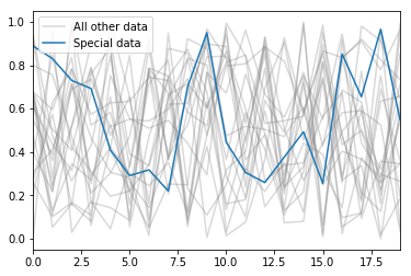
Advert: I do freelance data science work – please see here for more details.
↧
↧
Stack Abuse: Getting Started with Python PyAutoGUI
Introduction
In this tutorial, we're going to learn how to use pyautogui library in Python 3. The PyAutoGUI library provides cross-platform support for managing mouse and keyboard operations through code to enable automation of tasks. The pyautogui library is also available for Python 2; however, we will be using Python 3 throughout the course of this tutorial.
A tool like this has many applications, a few of which include taking screenshots, automating GUI testing (like Selenium), automating tasks that can only be done with a GUI, etc.
Before you go ahead with this tutorial, please note that there are a few prerequisites. You should have a basic understanding of Python's syntax, and/or have done at least beginner level programming in some other language. Other than that, the tutorial is quite simple and easy to follow for beginners.
Installation
The installation process for PyAutoGUI is fairly simple for all Operating Systems. However, there are a few dependencies for Mac and Linux that need to be installed before the PyAutoGUI library can be installed and used in programs.
Windows
For Windows, PyAutoGUI has no dependencies. Simply run the following command in your command prompt and the installation will be done.
$ pip install PyAutoGUI
Mac
For Mac, pyobjc-core and pyobjc modules are needed to be installed in sequence first. Below are the commands that you need to run in sequence in your terminal for successful installation:
$ pip3 install pyobjc-core
$ pip3 install pyobjc
$ pip3 install pyautogui
Linux
For Linux, the only dependency is python3-xlib (for Python 3). To install that, followed by pyautogui, run the two commands mentioned below in your terminal:
$ pip3 install python3-xlib
$ pip3 install pyautogui
Basic Code Examples
In this section, we are going to cover some of the most commonly used functions from the PyAutoGUI library.
Generic Functions
The position() Function
Before we can use PyAutoGUI functions, we need to import it into our program:
import pyautogui as pag
This position() function tells us the current position of the mouse on our screen:
pag.position()
Output:
Point (x = 643, y = 329)
The onScreen() Function
The onScreen() function tells us whether the point with coordinates x and y exists on the screen:
print(pag.onScreen(500, 600))
print(pag.onScreen(0, 10000))
Output:
True
False
Here we can see that the first point exists on the screen, but the second point falls beyond the screen's dimensions.
The size() Function
The size() function finds the height and width (resolution) of a screen.
pag.size()
Output:
Size (width = 1440, height = 900)
Your output may be different and will depend on your screen's size.
Common Mouse Operations
In this section, we are going to cover PyAutoGUI functions for mouse manipulation, which includes both moving the position of the cursor as well as clicking buttons automatically through code.
The moveTo() Function
The syntax of the moveTo() function is as follows:
pag.moveTo(x_coordinate, y_coordinate)
The value of x_coordinate increases from left to right on the screen, and the value of y_coordinate increases from top to bottom. The value of both x_coordinate and y_coordinate at the top left corner of the screen is 0.
Look at the following script:
pag.moveTo(0, 0)
pag.PAUSE = 2
pag.moveTo(100, 500) #
pag.PAUSE = 2
pag.moveTo(500, 500)
In the code above, the main focus is the moveTo() function that moves the mouse cursor on the screen based on the coordinates we provide as parameters. The first parameter is the x-coordinate and the second parameter is the y-coordinate. It is important to note that these coordinates represent the absolute position of the cursor.
One more thing that has been introduced in the code above is the PAUSE property; it basically pauses the execution of the script for the given amount of time. The PAUSE property has been added in the above code so that you can see the function execution; otherwise, the functions would execute in a split second and you wont be able to actually see the cursor moving from one location to the other on the screen.
Another workaround for this would be to indicate the time for each moveTo() operation as the third parameter in the function, e.g. moveTo(x, y, time_in_seconds).
Executing the above script may result in the following error:
Note: Possible Error
Traceback (most recent call last):
  File "a.py", line 5, in <module>
    pag.moveTo (100, 500)
  File "/anaconda3/lib/python3.6/site-packages/pyautogui/__init__.py", line 811, in moveTo
    _failSafeCheck()
  File "/anaconda3/lib/python3.6/site-packages/pyautogui/__init__.py", line 1241, in _failSafeCheck
    raise FailSafeException ('PyAutoGUI fail-safe triggered from mouse moving to a corner of the screen. To disable this fail-safe, set pyautogui.FAILSAFE to False. DISABLING FAIL-SAFE IS NOT RECOMMENDED.')
pyautogui.FailSafeException: PyAutoGUI fail-safe triggered from mouse moving to a corner of the screen. To disable this fail-safe, set pyautogui.FAILSAFE to False. DISABLING FAIL-SAFE IS NOT RECOMMENDED.
If the execution of the moveTo() function generates an error similar to the one shown above, it means that your computer's fail-safe is enabled. To disable the fail-safe, add the following line at the start of your code:
pag.FAILSAFE = False
This feature is enabled by default so that you can easily stop execution of your pyautogui program by manually moving the mouse to the upper left corner of the screen. Once the mouse is in this location, pyautogui will throw an exception and exit.
The moveRel() Function
The coordinates of the moveTo() function are absolute. However, if you want to move the mouse position relative to the current mouse position, you can use the moveRel() function.
What this means is that the reference point for this function, when moving the cursor, would not be the top left point on the screen (0, 0), but the current position of the mouse cursor. So, if your mouse cursor is currently at point (100, 100) on the screen and you call the moveRel() function with the parameters (100, 100, 2) the new position of your move cursor would be (200, 200).
You can use the moveRel() function as shown below:
pag.moveRel(100, 100, 2)
The above script will move the cursor 100 points to the right and 100 points down in 2 seconds, with respect to the current cursor position.
The click() Function
The click() function is used to imitate mouse click operations. The syntax for the click() function is as follows:
pag.click(x, y, clicks, interval, button)
The parameters are explained as follows:
x: the x-coordinate of the point to reachy: the y-coordinate of the point to reachclicks: the number of clicks that you would like to do when the cursor gets to that point on screeninterval: the amount of time in seconds between each mouse click i.e. if you are doing multiple mouse clicksbutton: specify which button on the mouse you would like to press when the cursor gets to that point on screen. The possible values areright,left, andmiddle.
Here is an example:
pag.click(100, 100, 5, 2, 'right')
You can also execute specific click functions as follows:
pag.rightClick(x, y)
pag.doubleClick(x, y)
pag.tripleClick(x, y)
pag.middleClick(x, y)
Here the x and y represent the x and y coordinates, just like in the previous functions.
You can also have more fine-grained control over mouse clicks by specifying when to press the mouse down, and when to release it up. This is done using the mouseDown and mouseUp functions, respectively.
Here is a short example:
pag.mouseDown(x=x, y=y, button='left')
pag.mouseUp(x=x, y=y, button='left')
The above code is equivalent to just doing a pag.click(x, y) call.
The scroll() Function
The last mouse function we are going to cover is scroll. As expected, it has two options: scroll up and scroll down. The syntax for the scroll() function is as follows:
pag.scroll(amount_to_scroll, x=x_movement, y=y_movement)
To scroll up, specify a positive value for amount_to_scroll parameter, and to scroll down, specify a negative value. Here is an example:
pag.scroll(100, 120, 120)
Alright, this was it for the mouse functions. By now, you should be able to control your mouse's buttons as well as movements through code. Let's now move to keyboard functions. There are plenty, but we will cover only those that are most frequently used.
Common Keyboard Operations
Before we move to the functions, it is important that we know which keys can be pressed through code in pyautogui, as well as their exact naming convention. To do so, run the following script:
print(pag.KEYBOARD_KEYS)
Output:
['\t', '\n', '\r', ' ', '!', '"', '#', '$', '%', '&', "'", '(', ')', '*', '+', ',', '-', '.', '/', '0', '1', '2', '3', '4', '5', '6', '7', '8', '9', ':', ';', '<', '=', '>', '?', '@', '[', '\\', ']', '^', '_', '`', 'a', 'b', 'c', 'd', 'e', 'f', 'g', 'h', 'i', 'j', 'k', 'l', 'm', 'n', 'o', 'p', 'q', 'r', 's', 't', 'u', 'v', 'w', 'x', 'y', 'z', '{', '|', '}', '~', 'accept', 'add', 'alt', 'altleft', 'altright', 'apps', 'backspace', 'browserback', 'browserfavorites', 'browserforward', 'browserhome', 'browserrefresh', 'browsersearch', 'browserstop', 'capslock', 'clear', 'convert', 'ctrl', 'ctrlleft', 'ctrlright', 'decimal', 'del', 'delete', 'divide', 'down', 'end', 'enter', 'esc', 'escape', 'execute', 'f1', 'f10', 'f11', 'f12', 'f13', 'f14', 'f15', 'f16', 'f17', 'f18', 'f19', 'f2', 'f20', 'f21', 'f22', 'f23', 'f24', 'f3', 'f4', 'f5', 'f6', 'f7', 'f8', 'f9', 'final', 'fn', 'hanguel', 'hangul', 'hanja', 'help', 'home', 'insert', 'junja', 'kana', 'kanji', 'launchapp1', 'launchapp2', 'launchmail', 'launchmediaselect', 'left', 'modechange', 'multiply', 'nexttrack', 'nonconvert', 'num0', 'num1', 'num2', 'num3', 'num4', 'num5', 'num6', 'num7', 'num8', 'num9', 'numlock', 'pagedown', 'pageup', 'pause', 'pgdn', 'pgup', 'playpause', 'prevtrack', 'print', 'printscreen', 'prntscrn', 'prtsc', 'prtscr', 'return', 'right', 'scrolllock', 'select', 'separator', 'shift', 'shiftleft', 'shiftright', 'sleep', 'space', 'stop', 'subtract', 'tab', 'up', 'volumedown', 'volumemute', 'volumeup', 'win', 'winleft', 'winright', 'yen', 'command', 'option', 'optionleft', 'optionright']
The typewrite() Function
The typewrite() function is used to type something in a text field. Syntax for the function is as follows:
pag.typewrite(text, interval)
Here text is what you wish to type in the field and interval is time in seconds between each key stroke. Here is an example:
pag.typewrite('Junaid Khalid', 1)
Executing the script above will enter the text "Junaid Khalid" in the field that is currently selected with a pause of 1 second between each key press.
Another way this function can be used is by passing in a list of keys that you'd like to press in a sequence. To do that through code, see the example below:
pag.typewrite(['j', 'u', 'n', 'a', 'i', 'd', 'e', 'backspace', 'enter'])
In the above example, the text junaide would be entered, followed by the removal of the trailing e. The input in the text field will be submitted by pressing the Enter key.
The hotkey() Function
If you haven't noticed this so far, the keys we've shown above have no mention for combined operations like Control + C for the copy command. In case you're thinking you could do that by passing the list ['ctrl', 'c'] to the typewrite() function, you are wrong. The typewrite() function would press both those buttons in a sequence, not simultaneously. And as you probably already know, to execute the copy command, you need to press the C key while holding the ctrl key.
To press two or more keys simultaneously, you can use the hotkey() function, as shown here:
pag.hotkey('shift', 'enter')
pag.hotkey('ctrl', '2' ) # For the @ symbol
pag.hotkey('ctrl', 'c')  # For the copy command
The screenshot() Function
If you would like to take a screenshot of the screen at any instance, the screenshot() function is the one you are looking for. Let's see how we can implement that using PyAutoGUI:
scree_shot = pag.screenshot() # to store a PIL object containing the image in a variable
This will store a PIL object containing the image in a variable.
If, however, you want to store the screenshot directly to your computer, you can call the screenshot function like this instead:
pag.screenshot('ss.png')
This will save the screenshot in a file, with the filename given, on your computer.
The confirm(), alert(), and prompt() Functions
The last set of functions that we are going to cover in this tutorial are the message box functions. Here is a list of the message box functions available in PyAutoGUI:
- Confirmation Box: Displays information and gives you two options i.e.
OKandCancel - Alert Box: Displays some information and to acknowledge that you have read it. It displays a single button i.e.
OK - Prompt Box: Requests some information from the user, and upon entering, the user has to click the
OKbutton
Now that we have seen the types, let's see how we can display these buttons on the screen in the same sequence as above:
pag.confirm("Are you ready?")
pag.alert("The program has crashed!")
pag.prompt("Please enter your name: ")
In the output, you will see the following sequence of message boxes.
Confirm:

Alert:

Prompt:

Conclusion
In this tutorial, we learned how to use PyAutoGUI automation library in Python. We started off by talking about pre-requisites for this tutorial, its installation process for different operating systems, followed by learning about some of its general function. After that we studied the functions specific to mouse movements, mouse control, and keyboard control.
After following this tutorial, you should be able to use PyAutoGUI to automate GUI operations for repetitive tasks in your own application.
↧
PyBites: Linting with Flake8
For so long the word "Linting" meant nothing to me. It sounded like some supercoder leet speak that was way out of my league. Then I discovered flake8 and realised I was a fool.
This article is a simple one. It covers what linting is; what Flake8 is and has an embarrassing example of it in use.
Before we get started, I need to get something off my chest. I don't know why but I really hate the word "linting". It's a hatred akin to people and the word "moist".
Linting. Linting. Linting. shudder. Let's move on!
What is Linting?
Just so I never have to type it again, let's quickly cover off what linting is.
It's actually pretty simple. Linting is the process of running a program that analyses code for programmatic errors such as bugs, actual errors, styling issues etc.
Put it in the same basket as the process running in your favourite text editor that keeps an eye out for typos and grammatical errors.
This brings us to Flake8.
What is Flake8?
It's one of these linting programs and is pretty damn simple to use. It also happens to analyse your code for PEP8 standard violations!
I love it for a few reasons:
- I'm constantly learning something new. It picks away at my code, pointing out my failings, much like annoying friends.
- It keeps my code looking schmick. It's easy to miss spacing and other tiny things while coding so running Flake8 against my code catches little annoyances before it's pushed to prod.
- It's a much nicer word than "linting".
Flake8 in Action
To demonstrate my beloved Flake8 I thought I'd grab an old, and I mean old, script that's likely riddled with issues. Judge me not friends!
In an older (I'm really stressing old here) article I wrote a simple script to send emails. No functions or anything, just line by line code. Ignoring what the code actually does take a look at this snippet below. Full code here.
λ cat generic_emailer.py
#!python3
#emailer.py is a simple script for sending emails using smtplib
#The idea is to assign a web-scraped file to the DATA_FILE constant.
#The data in the file is then read in and sent as the body of the email.

<snip>

DATA_FILE = 'scraped_data_file'
from_addr = 'your_email@gmail.com'
to_addr = 'your_email@gmail.com'  #Or any generic email you want all recipients to see
bcc = EMAILS

<snip>
Now that we have my script, let's run flake8 against it.
- pip install the sucker:
(venv) λ pip install flake8
- Simply run
flake8and point it at your script. Givengeneric_emailer.pyis in my current directory I'd run the following:
(venv) λ flake8 generic_emailer.py
- In traditional CLI fashion, if you don't receive any output at all, you have no issues. In my case, yeah, nope. The output I receive when running Flake8 against my script is as follows:
(venv) λ flake8 generic_emailer.py
generic_emailer.py:2:1: E265 block comment should start with '# '
generic_emailer.py:3:1: E265 block comment should start with '# '
generic_emailer.py:4:1: E265 block comment should start with '# '
generic_emailer.py:14:35: E262 inline comment should start with '# '
generic_emailer.py:14:80: E501 line too long (86 > 79 characters)
generic_emailer.py:27:50: E261 at least two spaces before inline comment
generic_emailer.py:27:51: E262 inline comment should start with '# '
generic_emailer.py:29:19: E261 at least two spaces before inline comment
generic_emailer.py:29:20: E262 inline comment should start with '# '
generic_emailer.py:31:23: E261 at least two spaces before inline comment
generic_emailer.py:31:24: E262 inline comment should start with '# '
generic_emailer.py:33:1: E265 block comment should start with '# '
generic_emailer.py:38:1: E265 block comment should start with '# '
generic_emailer.py:41:1: E265 block comment should start with '# '
generic_emailer.py:44:1: E265 block comment should start with '# '
Analysing the Output
Before we look into the actual issues, here's a quick breakdown of what the above means.
- The first section is the name of the file we're... flaking... Yes, I'm making the word "flaking" a thing!
- The next two numbers represent the line number and the character position in that line. ie: line 2, position 1.
- Finally, we have the actual issue. The "E" number is the error/violation number. The rest is the detail of the problem.
Now what does it all mean?
Well, the majority of my violations here have to do with the spacing in front of my comments.
- The E265 violations are simply telling me to add a space after my
#to satisfy standards. - E510 is saying I have too many characters in my line with the limit being 79.
You can read the rest!
Fixing the Violations
Let's quickly fix two of the violations:
generic_emailer.py:14:35: E262 inline comment should start with '# 'generic_emailer.py:14:80: E501 line too long (86 > 79 characters)
The code in question on line 14 is this:
to_addr = 'your_email@gmail.com' #Or any generic email you want all recipients to see
I can actually fix both issues by simply removing the comment. Doing this and running Flake8 again gets me the following output:
(venv) λ flake8 generic_emailer.py
generic_emailer.py:2:1: E265 block comment should start with '# '
generic_emailer.py:3:1: E265 block comment should start with '# '
generic_emailer.py:4:1: E265 block comment should start with '# '
generic_emailer.py:27:50: E261 at least two spaces before inline comment
generic_emailer.py:27:51: E262 inline comment should start with '# '
generic_emailer.py:29:19: E261 at least two spaces before inline comment
generic_emailer.py:29:20: E262 inline comment should start with '# '
generic_emailer.py:31:23: E261 at least two spaces before inline comment
generic_emailer.py:31:24: E262 inline comment should start with '# '
generic_emailer.py:33:1: E265 block comment should start with '# '
generic_emailer.py:38:1: E265 block comment should start with '# '
generic_emailer.py:41:1: E265 block comment should start with '# '
generic_emailer.py:44:1: E265 block comment should start with '# '
Note the two violations are gone.
Ignoring Violations
What if I don't care about the spacing of my comment #s?
Sometimes you'll want Flake8 to ignore specific issues. One of the most common use cases is to ignore line length.
You can do this by running flake8 --ignore=E<number>. Just specify which violations you want to ignore and Flake8 will overlook them.
To save yourself time you can also create a Flake8 config file and hardcode the violation codes into that. This method will save you specifying the code every time you run Flake8.
In my case I'm going to ignore those pesky E265 violations because I can.
I need to create a .flake8 file in my parent directory and add the following (with vim of course!):
(venv) λ touch flake8
(venv) λ cat .flake8
[flake8]
ignore = E265
When I re-run Flake8 I now see the following:
(venv) λ flake8 generic_emailer.py
generic_emailer.py:27:50: E261 at least two spaces before inline comment
generic_emailer.py:27:51: E262 inline comment should start with '# '
generic_emailer.py:29:19: E261 at least two spaces before inline comment
generic_emailer.py:29:20: E262 inline comment should start with '# '
generic_emailer.py:31:23: E261 at least two spaces before inline comment
generic_emailer.py:31:24: E262 inline comment should start with '# '
The rest of the errors are an easy clean up so I'll leave it here.
Flake8 on PyBites CodeChallenges
As luck would have it, we've just implemented a new feature on the PyBites CodeChallenges platform that allows you to run flake8 against your browser based code!
Now you can have flake8 lint your code to perfection while you solve our Bites.
Check it out in all its glory:

Conclusion
Whether you like the word Linting or not, there's no denying the value it can provide - Flake8 case in point.
While it can definitely grow a little tiresome at times if you have a well crafted config file you can customise it to your liking and pain threshold.
It really is a brilliant tool to add to your library so give it a try!
Keep Calm and Code in Python!
-- Julian
↧
Real Python: Get Started With Django: Build a Portfolio App
Django is a fully featured Python web framework that can be used to build complex web applications. In this course, you’ll jump in and learn Django by example. You’ll follow the steps to create a fully functioning web application and, along the way, learn some of the most important features of the framework and how they work together.
By the end of this course, you will be able to:
- Understand what Django is and why it’s a great web framework
- Understand the architecture of a Django site and how it compares with other frameworks
- Set up a new Django 2 project and app
- Build a personal portfolio website with Django 2 and Python 3
[ Improve Your Python With 🐍 Python Tricks 💌 – Get a short & sweet Python Trick delivered to your inbox every couple of days. >> Click here to learn more and see examples ]
↧
↧
PyCharm: Webinar Preview: Project Setup for React+TS+TDD
Next Wednesday (Oct 16) I’m giving a webinar on React+TypeScript+TDD in PyCharm. Let’s give a little background on the webinar and spotlight one of the first parts covered.

Background
Earlier this year we announced a twelve-part in-depth tutorial on React, TypeScript, and Test-Driven Development (TDD) in PyCharm. For the most part it highlights PyCharm Professional’s bundling of WebStorm, our professional IDE for web development.
The tutorial is unique in a few ways:
- It’s React, but with TypeScript, a combination with spotty coverage
- Concepts are introduced through the lens of test-driven development, where you explore in the IDE, not the browser
- Each tutorial step has a narrated video plus an in-depth discussion with working code
- The tutorial highlights places where the IDE does your janitorial work for you and helps you “fail faster” and stay in the “flow”
This webinar will cover sections of that tutorial in a “ask-me-anything” kind of format. There’s no way we’ll get through all the sections, but we’ll get far enough give attendees a good grounding on the topic. As a note, I’m also later giving this tutorial later as a guest for both an IntelliJ IDEA webinar and Rider webinar.
I really enjoy telling the story about combining TypeScript with TDD to “fail faster”, as well as letting the IDE do your janitorial work to help you stay in the “flow.” Hope you’ll join us!
Spotlight: Project Setup
The tutorial starts with Project Setup, which uses the IDE’s integration with Create React App to scaffold a React+TypeScript project. Note: The tutorial is, as is common in the world of JS, six months out of date. Things have changed, such as tslint -> eslint. I’ll re-record once PyCharm 2019.3 is released, but for the webinar, I’ll use the latest Create React App.
For this tutorial I started with an already-generated directory, but in the webinar I’ll show how to use the IDE’s New Project to do so.
This tutorial step orients us in the IDE: opening package.json to run scripts in tool windows, generating a production build, and running a test then re-running it after an edit.
The second tutorial step does some project cleanup before getting into testing.
↧
Codementor: Python-compatible IDEs: What is It and Why Do You Need It?
There is no better way to build in Python than by using an IDE (Integrated Development Environment). They not only make your work much easier as well as logical; they also enhance the coding...
↧
Python Circle: Solving Python Error- KeyError: 'key_name'
Solving KeyError in python, How to handle KeyError in python dictionary, Safely accessing and deleting keys from python dictionary, try except Key error in Python
↧
Python Circle: 5 lesser used Django template tags
rarely used Django template tags, lesser-known Django template tags, 5 awesome Django template tags, Fun with Django template tags,
↧
↧
PyCoder’s Weekly: Issue #389 (Oct. 8, 2019)
#389 – OCTOBER 8, 2019
View in Browser »
Get Started With Django: Build a Portfolio App
In this course, you’ll learn the basics of creating powerful web applications with Django, a Python web framework. You’ll build a portfolio website to showcase your web development projects, complete with a fully functioning blog.
REAL PYTHONvideo
Auto Formatters for Python
An auto formatter is a tool that will format your code in a way it complies with the tool or any other standard it set. But which auto formatter should you use with Python code?
KEVIN PETERS• Shared by Kevin Peters
Monitor Your Python Applications With Datadog’s Distributed Tracing and APM
Debug and optimize your code by tracing requests across web servers, databases, and services in your environment—and seamlessly correlate those traces with metrics and logs to troubleshoot issues. Try Datadog in your environment with a free 14-day trial →
DATADOGsponsor
Timsort: The Fastest Sorting Algorithm You’ve Never Heard Of
CPython uses Timsort for sorting containers. Timsort is a fast O(n log n) stable sorting algorithm built for the real world — not constructed in academia.
BRANDON SKERRITT
PyPy’s New JSON Parser
PyPy has a new and faster JSON parser implementation. This post covers the design decisions that were made to develop the new and improved parser.
PYPY STATUS BLOG
Automatically Reloading Python Modules With %autoreload
Tired of having to reload a module each time you change it? IPython’s %autoreload to the rescue!
SEBASTIAN WITOWSKI
Six Django Template Tags Not Often Used in Tutorials
{% for ... %} {% empty %} {% endfor %} anyone?
MEDIUM.COM/@HIGHCENBURG
(Floating Point) Numbers, They Lie
When and why 2 + 2 = 4.00000000000000000001…
GLYPH LEFKOWITZ
Discussions
What’s Your Favorite Python Library?
Twitter discussion about everyone’s best-loved Python libraries. What’s your personal favorite?
MIKE DRISCOLL
Python Jobs
Full Stack Developer (Toronto, ON, Canada)
Backend Developer (Kfar Saba, Israel)
Articles & Tutorials
How Dictionaries Are Implemented in CPython
Learn what hash tables are, why you would use them, and how they’re used to implement dictionaries in the most popular Python interpreter: CPython.
DATA-STRUCTURES-IN-PRACTICE.COM
Building a Python C Extension Module
Learn how to write Python interfaces in C. Find out how to invoke C functions from within Python and build Python C extension modules. You’ll learn how to parse arguments, return values, and raise custom exceptions using the Python API.
REAL PYTHON
Automated Python Code Reviews, Directly From Your Git Workflow
Codacy lets developers spend more time shipping code and less time fixing it. Set custom standards and automatically track quality measures like coverage, duplication, complexity and errors. Integrates with GitHub, GitLab and Bitbucket, and works with 28 different languages. Get started today for free →
CODACYsponsor
Is Rectified Adam Actually Better Than Adam?
“Is the Rectified Adam (RAdam) optimizer actually better than the standard Adam optimizer? According to my 24 experiments, the answer is no, typically not (but there are cases where you do want to use it instead of Adam).”
ADRIAN ROSEBROCK
Using the Python zip() Function for Parallel Iteration
How to use Python’s built-in zip() function to solve common programming problems. You’ll learn how to traverse multiple iterables in parallel and create dictionaries with just a few lines of code.
REAL PYTHON
How Is Python 2 Supported in RHEL After 2020?
What the Py 2.x end-of-life deadline means in practice, e.g. “Just because the PSF consider Python 2 unsupported does not mean that Python 2 is unsupported within RHEL.” Also see the related discussion on Hacker News.
REDHAT.COM
Principal Component Analysis (PCA) With Python, From Scratch
Derive PCA from first principles and implement a working version in Python by writing all the linear algebra code from scratch. Nice tutorial!
ORAN LOONEY
Winning the Python Software Interview
Tips on acing your Python coding interview, PSF has a new Code of Conduct, and regex testing tools.
PYTHON BYTES FMpodcast
Analyzing the Stack Overflow Survey With Python and Pandas
Do your own data science exploration and analysis on the annual developer survey’s dataset.
MOSHE ZADKA
Python 2 EOL: Are You Prepared? Take Our Survey for a Chance to Win a Drone!
Python 2 End of Life is coming soon. Please take our 5-minute survey to let us know how you’re preparing for the change. You’ll get the final results, plus the chance to win a camera drone. Thanks for your time!
ACTIVESTATEsponsor
How to Add Maps to Django Web App Projects With Mapbox
Learn how to add maps and location-based data to your web applications using Mapbox.
MATT MAKAI
Projects & Code
Events
SciPy Latam
October 8 to October 11, 2019
SCIPYLA.ORG
PyCon ZA 2019
October 9 to October 14, 2019
PYCON.ORG
PyConDE & PyData Berlin 2019
October 9 to October 12, 2019
PYCON.ORG
Python Miami
October 12 to October 13, 2019
PYTHONDEVELOPERSMIAMI.COM
PyCon Pakistan 2019
October 12 to October 13, 2019
PYCON.PK
PyCon India 2019
October 12 to October 16, 2019
PYCON.ORG
PyCode Conference 2019
October 14 to October 17, 2019
PYCODE-CONFERENCE.ORG
Happy Pythoning!
This was PyCoder’s Weekly Issue #389.
View in Browser »
[ Subscribe to 🐍 PyCoder’s Weekly 💌 – Get the best Python news, articles, and tutorials delivered to your inbox once a week >> Click here to learn more ]
↧
PyPy Development: PyPy's new JSON parser
Introduction
In the last year or two I have worked on and off on making PyPy's JSON faster, particularly when parsing large JSON files. In this post I am going to document those techniques and measure their performance impact. Note that I am quite a lot more constrained in what optimizations I can apply here, compared to some of the much more advanced approaches like Mison, Sparser or SimdJSON because I don't want to change the json.loads API that Python programs expect, and because I don't want to only support CPUs with wide SIMD extensions. With a more expressive API, more optimizations would be possible.There are a number of problems of working with huge JSON files: deserialization takes a long time on the one hand, and the resulting data structures often take a lot of memory (usually they can be many times bigger than the size of the file they originated from). Of course these problems are related, because allocating and initializing a big data structure takes longer than a smaller data structure. Therefore I always tried to attack both of these problems at the same time.
One common theme of the techniques I am describing is that of optimizing the parser for how JSON files are typically used, not how they could theoretically be used. This is a similar approach to the way dynamic languages are optimized more generally: most JITs will optimize for typical patterns of usage, at the cost of less common usage patterns, which might even become slower as a result of the optimizations.
Maps
The first technique I investigated is to use maps in the JSON parser. Maps, also called hidden classes or shapes, are a fairly common way to (generally, not just in the context of JSON parsing) optimize instances of classes in dynamic language VMs. Maps exploit the fact that while it is in theory possible to add arbitrary fields to an instance, in practice most instances of a class are going to have the same set of fields (or one of a small number of different sets). Since JSON dictionaries or objects often come from serialized instances of some kind, this property often holds in JSON files as well: dictionaries often have the same fields in the same order, within a JSON file.This property can be exploited in two ways: on the one hand, it can be used to again store the deserialized dictionaries in a more memory efficient way by not using a hashmap in most cases, but instead splitting the dictionary into a shared description of the set of keys (the map) and an array of storage with the values. This makes the deserialized dictionaries smaller if the same set of keys is repeated a lot. This is completely transparent to the Python programmer, the dictionary will look completely normal to the Python program but its internal representation is different.
One downside of using maps is that sometimes files will contain many dictionaries that have unique key sets. Since maps themselves are quite large data structures and since dictionaries that use maps contain an extra level of indirection we want to fall back to using normal hashmaps to represent the dictionaries where that is the case. To prevent this we perform some statistics at runtime, how often every map (i.e. set of keys) is used in the file. For uncommonly used maps, the map is discarded and the dictionaries that used the map converted into using a regular hashmap.
Using Maps to Speed up Parsing
Another benefit of using maps to store deserialized dictionaries is that we can use them to speed up the parsing process itself. To see how this works, we need to understand maps a bit better. All the maps produced as a side-effect of parsing JSON form a tree. The tree root is a map that describes the object without any attributes. From every tree node we have a number of edges going to other nodes, each edge for a specific new attribute added:This map tree is the result of parsing a file that has dictionaries with the keys a, b, c many times, the keys a, b, f less often, and also some objects with the keys x, y.
When parsing a dictionary we traverse this tree from the root, according to the keys that we see in the input file. While doing this, we potentially add new nodes, if we get key combinations that we have never seen before. The set of keys of a dictionary parsed so far are represented by the current tree node, while we can store the values into an array. We can use the tree of nodes to speed up parsing. A lot of the nodes only have one child, because after reading the first few keys of an object, the remaining ones are often uniquely determined in a given file. If we have only one child map node, we can speculatively parse the next key by doing a memcmp between the key that the map tree says is likely to come next and the characters that follow the ',' that started the next entry in the dictionary. If the memcmp returns true this means that the speculation paid off, and we can transition to the new map that the edge points to, and parse the corresponding value. If not, we fall back to general code that parses the string, handles escaping rules etc. This trick was explained to me by some V8 engineers, the same trick is supposedly used as part of the V8 JSON parser.
This scheme doesn't immediately work for map tree nodes that have more than one child. However, since we keep statistics anyway about how often each map is used as the map of a parsed dictionary, we can speculate that the most common map transition is taken more often than the others in the future, and use that as the speculated next node.
So for the example transition tree shown in the figure above the key speculation would succeed for objects with keys a, b, c. For objects with keys a, b, f the speculation would succeed for the first two keys, but not for the third key f. For objects with the keys x, y the speculation would fail for the first key x but succeed for the second key y.
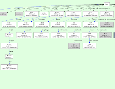
For real-world datasets these transition trees can become a lot more complicated, for example here is a visualization of a part of the transition tree generated for parsing a New York Times dataset:
Caching Strings
A rather obvious observation we can use to improve performance of the parser is the fact that string values repeat a lot in most JSON files. For strings that are used as dictionary keys this is pretty obvious. However it happens also for strings that are used as values in dictionaries (or are stored in lists). We can use this fact to intern/memoize strings and save memory. This is an approach that many JSON parsers use, including CPython's. To do this, I keep a dictionary of strings that we have seen so far during parsing and look up new strings that are deserialized. If we have seen the string before, we can re-use the deserialized previous string. Right now I only consider utf-8 strings for caching that do not contain any escapes (whether stuff like \", \n or escaped unicode chars).This simple approach works extremely well for dictionary keys, but needs a number of improvements to be a win in general. The first observation is that computing the hash to look up the string in the dictionary of strings we've seen so far is basically free. We can compute the hash while scanning the input for the end of the string we are currently deserializing. Computing the hash while scanning doesn't increase the time spent scanning much. This is not a new idea, I am sure many other parsers do the same thing (but CPython doesn't seem to).
Another improvement follows from the observation that inserting every single deserialized non-key string into a hashmap is too expensive. Instead, we insert strings into the cache more conservatively, by keeping a small ring buffer of hashes of recently deserialized strings. The hash is looked for in the ring buffer, and only if the hash is present we insert the string into the memoization hashmap. This has the effect of only inserting strings into the memoization hashmap that re-occur a second time not too far into the file. This seems to give a good trade-off between still re-using a lot of strings but keeping the time spent updating and the size of the memoization hashmap low.
Another twist is that in a lot of situations caching strings is not useful at all, because it will almost never succeed. Examples of this are UUIDs (which are unique), or the content of a tweet in a JSON file with many tweets (which is usually unique). However, in the same file it might be useful to cache e.g. the user name of the Twitter user, because many tweets from the same person could be in such a file. Therefore the usefulness of the string cache depends on which fields of objects we are deserializing the value off. Therefore we keep statistics per map field and disable string memoization per individual field if the cache hit rate falls below a certain threshold. This gives the best of both worlds: in the cases where string values repeat a lot in certain fields we use the cache to save time and memory. But for those fields that mostly contain unique strings we don't waste time looking up and adding strings in the memoization table. Strings outside of dictionaries are quite rare anyway, so we just always try to use the cache for them.
The following pseudocode sketches the code to deserialize a string in the input at a given position. The function also takes a map, which is the point in the map tree that we are currently deserializing a field off (if we are deserializing a string in another context, some kind of dummy map can be used there).
def deserialize_string(pos, input, map):
    # input is the input string, pos is the position of the starting " of
    # the string

    # find end of string, check whether it contains escape codes,
    # compute hash, all at the same time
    end, escapes, hash = find_end_of_string(pos + 1, input)
    if end == -1:
        raise ParseError
    if escapes:
        # need to be much more careful with escaping
        return deserialize_string_escapes(pos, input)

    # should we cache at all?
    if map.cache_disabled():
        return input[pos + 1:end]

    # if string is in cache, return it
    if hash in cache:
        map.cache_hit += 1
        return cache[hash]

    result = input[pos + 1:end]
    map.cache_miss += 1

    # if hash is in the ring buffer of recently seen hashes,
    # add the string to the cache
    if hash in ring_buffer:
        cache[hash] = result
    else:
        ring_buffer.write(hash)
    return result
Evaluation
To find out how much the various techniques help, I implemented a number of JSON parsers in PyPy with different combinations of the techniques enabled. I compared the numbers with the JSON parser of CPython 3.7.3 (simplejson), with ujson, with the JSON parser of Node 12.11.1 (V8) and with RapidJSON (in DOM mode).I collected a number of medium-to-large JSON files to try the JSON parsers on:
- Censys: A subset of the Censys port and protocol scan data for websites in the Alexa top million domains
- Gharchive: Github activity from January 15-23, 2015 from Github Archive
- Reddit: Reddit comments from May 2009
- Rosie: The nested matches produced using the Rosie pattern languageall.things pattern on a log file
- Nytimes: Metadata of a collection of New York Times articles
- Tpch: The TPC-H database benchmark's deals table as a JSON file
- Twitter: A JSON export of the @pypyproject Twitter account data
- Wikidata: A file storing a subset of the Wikidata fact dump from Nov 11, 2014
- Yelp: A file of yelp businesses
| Benchmark | File Size [MiB] |
|---|---|
| Censys | 898.45 |
| Gharchive | 276.34 |
| NYTimes | 12.98 |
| 931.65 | |
| Rosie | 388.88 |
| TPCH | 173.86 |
| Wikidata | 119.75 |
| Yelp | 167.61 |
- PyPyBaseline: The PyPy JSON parser as it was before my work with JSON parsing started (PyPy version 5.8)
- PyPyKeyStringCaching: Memoizing the key strings of dictionaries, but not the other strings in a json file, and not using maps to represent dictionaries (this is the JSON parser that PyPy has been shipping since version 5.9, in the benchmarks I used 7.1).
- PyPyMapNoCache: Like PyPyKeyStringCaching, but using maps to represent dictionaries. This includes speculatively parsing the next key using memcmp, but does not use string caching of non-key strings.
- PyPyFull: Like PyPyMapNoCache but uses a string cache for all strings, not just keys. This is equivalent to what will be released soon as part of PyPy 7.2
Contributions of Individual Optimizations
Let's first look at the contributions of the individual optimizations to the overall performance and memory usage.All the benchmarks were run 30 times in new processes, all the numbers are normalized to PyPyFull.
The biggest individual improvement to both parsing time and memory used comes from caching just the keys in parsed dictionaries. This is the optimization in PyPy's JSON parser that has been implemented for a while already. To understand why this optimization is so useful, let's look at some numbers about each benchmark, namely the number of total keys across all dictionaries in each file, as well as the number of unique keys. As we can see, for all benchmarks the number of unique keys is significantly smaller than the number of keys in total.
| Benchmark | Number of keys | Number of unique keys |
|---|---|---|
| Censys | 14 404 234 | 163 |
| Gharchive | 6 637 881 | 169 |
| NYTimes | 417 337 | 60 |
| 25 226 397 | 21 | |
| Rosie | 28 500 101 | 5 |
| TPCH | 6 700 000 | 45 |
| Wikidata | 6 235 088 | 1 602 |
| Yelp | 5 133 914 | 61 |
We can look at some numbers about every benchmark again. The table shows how many map-based dictionaries are deserialized for every benchmark, and how many hashmap-backed dictionaries. We see that the number of hashmap-backed dictionaries is often zero, or at most a small percentage of all dictionaries in each benchmark. Yelp has the biggest number of hashmap-backed dictionaries. The reason for this is that the input file contains hashmaps that store combinations of various features of Yelp businesses, and a lot of these combinations are totally unique to a business. Therefore the heuristics determine that it's better to store these using hashmaps.
| Benchmark | Map Dicts | Regular Dicts | % Regular Dicts |
|---|---|---|---|
| Censys | 4 049 235 | 1 042 | 0.03 |
| Gharchive | 955 301 | 0 | 0.00 |
| NYTimes | 80 393 | 0 | 0.00 |
| 1 201 257 | 0 | 0.00 | |
| Rosie | 6 248 966 | 0 | 0.00 |
| TPCH | 1 000 000 | 0 | 0.00 |
| Wikidata | 1 923 460 | 46 905 | 2.38 |
| Yelp | 443 140 | 52 051 | 10.51 |
| Benchmark | Number of Keys | Map Transitions | % Successful Speculation |
|---|---|---|---|
| Censys | 14 404 234 | 14 403 243 | 65.79 |
| Gharchive | 6 637 881 | 6 637 881 | 86.71 |
| NYTimes | 417 337 | 417 337 | 79.85 |
| 25 226 397 | 25 226 397 | 100.00 | |
| Rosie | 28 500 101 | 28 500 101 | 90.37 |
| TPCH | 6 700 000 | 6 700 000 | 86.57 |
| Wikidata | 6 235 088 | 5 267 744 | 63.68 |
| Yelp | 5 133 914 | 4 593 980 | 90.43 |
| geomean | 82.04 |
Comparison against other JSON Decoders
To get a more general feeling of the performance and memory usage of the improved PyPy parser, we compare it against CPython's built-in json parser, ujson for CPython, Node's (V8) JSON parser and RapidJSON. For better context for the memory usage I also show the file size of the input files.These benchmarks are not really an apples-to-apple comparison. All of the implementations use different in-memory representations of strings in the deserialized data-structure (Node uses two bytes per character in a string, in CPython it depends but 4 bytes on my machine), PyPyBaseline uses four bytes, PyPy and RapidJSON use utf-8). But it's still interesting to get some ballpark numbers. The results are as follows:
As we can see, PyPyFull handily beats CPython and ujson, with a geometric mean of the improvement of about 2.5×. The memory improvement can be even more extreme, with an improvement of over 4× against CPython/ujson in some cases (CPython gives better memory sizes, because its parser caches the keys of dictionaries as well). Node is often more than 50% slower, whereas RapidJSON beats us easily, by a factor of 2× on average.
Conclusions
While the speedup I managed to achieve over the course of this project is nice and I am certainly happy to beat both CPython and Node, I am ultimately still annoyed that RapidJSON manages to maintain such a clear lead over PyPyFull, and would like to get closer to it. One problem that PyPy suffers compared to RapidJSON is the overhead of garbage collection. Deserializing large JSON files is pretty much the worst case for the generational GC that PyPy uses, since none of the deserialized objects die young (and the GC expects that most objects do). That means that a lot of the deserialization time of PyPy is wasted allocating the resulting objects in the nursery, and then copying them into the old generation. Somehow, this should be done in better ways, but all my attempts to not have to do the copy did not seem to help much. So maybe more improvements are possible, if I can come up with more ideas.On the memory side of things, Node/V8 is beating PyPy clearly which might indicate more general problems in how we represent Python objects in memory. On the other hand, I think it's cool that we are competitive with RapidJSON in terms of memory and often within 2× of the file size.
An effect that I didn't consider at all in this blog post is the fact that accessing the deserialized objects with constants strings is also faster than with regular dictionaries, due to them being represented with maps. More benchmarking work to do in the future!
If you have your own programs that run on PyPy and use the json parser a lot, please measure them on the new code and let me know whether you see any difference!
↧
Wingware News: Wing Python IDE 7.1.2 - October 7, 2019
Wing 7.1.2 adds a How-To for using Wing with Docker, allows disabling code warnings from the tooltip displayed over the editor, adds support for macOS 10.15 (Catalina), supports code folding in JSON files, adds optional word wrapping for output in the Testing tool, and fixes about 25 minor usability issues.

Download Wing 7.1.2 Now:Wing Pro | Wing Personal | Wing 101 | Compare Products
![]() Some Highlights of Wing 7.1
Some Highlights of Wing 7.1
 Some Highlights of Wing 7.1
Support for Python 3.8
Wing 7.1 supports editing, testing, and debugging code written for Python 3.8, so you can take advantage of assignment expressions and other improvements introduced in this new version of Python.
Improved Code Warnings
Wing 7.1 adds unused symbol warnings for imports, variables, and arguments found in Python code. This release also improves code warnings configuration, making it easier to disable unwanted warnings.
Cosmetic Improvements
Wing 7.1 improves the auto-completer, project tool, and code browser with redesigned icons that make use of Wing's icon color configuration. This release also improves text display on some Linux systems, supports Dark Mode on macOS, and improves display of Python code and icons found in documentation.
And More
Wing 7.1 also adds a How-To for using Wing with Docker, the ability to disable code warnings from tooltips on the editor, support for macOS 10.15 (Catalina), code folding in JSON files, word wrapping for output in the Testing tool, support for Windows 10 native OpenSSH installations for remote development, and many minor improvements. This release drops support for macOS 10.11. System requirements remain unchanged on Windows and Linux.
For details see the change log.
For a complete list of new features in Wing 7, see What's New in Wing 7.
![]() Try Wing 7.1 Now!
Try Wing 7.1 Now!
Wing 7.1 is an exciting new step for Wingware's Python IDE product line. Find out how Wing 7.1 can turbocharge your Python development by trying it today.
Downloads:Wing Pro | Wing Personal | Wing 101 | Compare Products
See Upgrading for details on upgrading from Wing 6 and earlier, and Migrating from Older Versions for a list of compatibility notes.
↧
Python Insider: Python 2.7.17 release candidate 1 available
↧
↧
Python Engineering at Microsoft: Announcing Support for Native Editing of Jupyter Notebooks in VS Code
With today’s October release of the Python extension, we’re excited to announce the support of native editing of Jupyter notebooks inside Visual Studio Code! You can now directly edit .ipynb files and get the interactivity of Jupyter notebooks with all of the power of VS Code. You can manage source control, open multiple files, and leverage productivity features like IntelliSense, Git integration, and multi-file management, offering a brand-new way for data scientists and developers to experiment and work with data efficiently. You can try out this experience today by downloading the latest version of the Python extension and creating/opening a Jupyter Notebook inside VS Code.

Since the initial release of our data science experience in VS Code, one of the top features that users have requested has been a more notebook-like layout to edit their Jupyter notebooks inside VS Code. In the rest of this post we’ll take a look at the new capabilities this offers.
Getting Started
Here’s how to get started with Jupyter in VS Code.
- If you don’t already have an existing Jupyter Notebook file, open the VS Code Command Palette with the shortcut CTRL + SHIFT + P (Windows) or Command + SHIFT + P (macOS), and run the “Python: Create Blank New Jupyter Notebook” command.
- If you already have a Jupyter Notebook file, it’s as simple as just opening that file in VS Code. It will automatically open with the new native Jupyter editor.

Once you have a Jupyter Notebook open, you can add new cells, write code in cells, run cells, and perform other notebook actions.
AI-Assisted Autocompletion
As you write code, IntelliSense will give you intelligent code complete suggestions right inside your code cells. You can further supercharge your editor experience by installing our IntelliCode extension to get AI-powered IntelliSense with smarter auto-complete suggestions based on your current code context.

Variable Explorer
Another benefit of using VS Code is that you can take advantage of the variable explorer and plot viewer by clicking the “Variables” button in the notebook toolbar. The variable explorer will help you keep track of the current state of your notebook variables at a glance, in real-time.

Now you can explore your datasets, filter your data, and even export plots! Gone are the days of having to type df.head() just to view your data.
Connecting To Remote Jupyter Servers
When a Jupyter notebook file is created or opened, VS Code automatically creates a Jupyter server for you locally by default. If you want to use a remote Jupyter server, it’s as simple as using the “Specify Jupyter server URI” command via the VS Code command palette, and entering in the server URI.

Exporting as Python Code
When you’re ready to turn experimentation into production-ready Python code, just simply press the “Convert and Save as Python File” button in the top toolbar and let the Python extension do all the work for you. You can then view that Python code in our existing Python Interactive window and keep on working with the awesome features of the Python extension to further make your code production-ready, such as the integrated debugger, refactoring, Visual Studio Live Share, and Git source control.

Debugging
VS Code supports debugging Jupyter Notebooks through using the “Exporting as Python Code” functionality outlined in the previous section. Once you have your code in the Python Interactive window, you can use VS Code’s integrated debugger to debug your code. We are working on bringing cell debugging into the Jupyter editor in a future release so stay tuned!
Try it out today!
You can check out the documentation for the full list of features available in the first release of the native Jupyter experience and learn to get started with Jupyter notebooks in VS Code. Also, if you have any suggestions or run across any issues, please file an issue in the Python extension GitHub page.
We’re excited for everyone to try out this new experience and have the Python extension in VS Code empower your notebook development!
The post Announcing Support for Native Editing of Jupyter Notebooks in VS Code appeared first on Python.
↧
Python Engineering at Microsoft: Python in Visual Studio Code – October 2019 Release
We are pleased to announce that the October 2019 release of the Python Extension for Visual Studio Code is now available. You can download the Python extension from the Marketplace, or install it directly from the extension gallery in Visual Studio Code. If you already have the Python extension installed, you can also get the latest update by restarting Visual Studio Code. You can learn more about Python support in Visual Studio Code in the documentation.
In this release we addressed 97 issues, including native editing of Jupyter Notebooks, a button to run a Python file in the terminal, and linting and import improvements with the Python Language Server. The full list of enhancements is listed in our changelog.
Native editing of Jupyter Notebooks
We’re excited to announce the first release of native editing of Jupyter notebooks inside VS Code! The native Jupyter experience brings a new way for both data scientists and notebook developers alike to directly edit .ipynb files and get the interactivity of Jupyter notebooks with all of the power of VS Code. You can check the blog post to learn more about this feature and how to get started.

Run Python File in Terminal button
This release includes a “play” button to run the Run Python File in Terminal command. Now it only takes one click to run Python files with the Python extension!
The new button is located on the top-right side of the editor, matching the behavior of the Code Runner extension:


If you’re into key bindings, you can also customize your own keyboard shortcut to run Python files in the terminal, by running the Preferences: Open Keyboard Shortcuts (JSON) command in the command palette (View > Command Palette…) and entering a key binding for the python.execInTerminal command as you prefer. For example, you could have the following definition to run Python files in the terminal with a custom shortcut:

If the Code Runner extension is enabled, the Python extension doesn’t display this button in order to avoid possible confusion.
Linting and import improvements with the Python Language Server
This release also includes three new linting rules with the Python Language Server, as well as significant improvements to autocompletion for packages such as PyTorch and pandas.
Additionally, there have been large improvements made to import resolution. Historically the Language Server has treated the workspace root as the sys.path entry (i.e. the main workspace root) of user module imports, which led to false-positive unresolved imports warnings when importing modules from a src directory. With this release, if there’s such a src directory in the project’s environment, the Language Server automatically detects and adds the directory to its list of search paths. You can refer to the documentation to learn more about configuring search paths for the Language Server.
Other Changes and Enhancements
We have also added small enhancements and fixed issues requested by users that should improve your experience working with Python in Visual Studio Code. Some notable changes include:
- Fix for test discovery issues with pytest 5.1+. (#6990)
- Fixes for detecting the shell. (#6928)
- Opt insiders users into the Beta version of the Language Server by default. (#7108)
- Replaced occurrences of pep8 with pycodestyle. All mentions of pep8 have been replaced with pycodestyle (thanks Marsfan). (#410)
We are continuing to A/B test new features. If you see something different that was not announced by the team, you may be part of the experiment! To see if you are part of an experiment, you can check the first lines in the Python extension output channel. If you wish to opt-out from A/B testing, you can open the user settings.json file (View > Command Palette… and run Preferences: Open Settings (JSON)) and set the “python.experiments.enabled” setting to false.
Be sure to download the Python extension for Visual Studio Code now to try out the above improvements. If you run into any problems, please file an issue on the Python VS Code GitHub page.
The post Python in Visual Studio Code – October 2019 Release appeared first on Python.
↧
Ned Batchelder: Pytest-cov support for who-tests-what
I’ve added a new option to the pytest-cov coverage plugin for pytest: --cov-context=test will set the dynamic context based on pytest test phases. Each test has a setup, run, and teardown phase. This gives you the best test information in the coverage database:
- The full test id is used in the context. You have the test file name, and the test class name if you are using class-based tests.
- Parameterized tests start a new context for each new set of parameter values.
- Execution is a little faster because coverage.py doesn’t have to poll for test starts.
For example, here is a repo of simple pytest tests in a number of forms: pytest-gallery. I can run the tests with test contexts being recorded:
$ pytest -v --cov=. --cov-context=test
======================== test session starts =========================
platform darwin -- Python 3.6.9, pytest-5.2.1, py-1.8.0, pluggy-0.12.0 -- /usr/local/virtualenvs/pytest-cov/bin/python3.6

cachedir: .pytest_cache

rootdir: /Users/ned/lab/pytest-gallery

plugins: cov-2.8.1

collected 25 items


test_fixtures.py::test_fixture PASSED                          [  4%]
test_fixtures.py::test_two_fixtures PASSED                     [  8%]
test_fixtures.py::test_with_expensive_data PASSED              [ 12%]
test_fixtures.py::test_with_expensive_data2 PASSED             [ 16%]
test_fixtures.py::test_parametrized_fixture[1] PASSED          [ 20%]
test_fixtures.py::test_parametrized_fixture[2] PASSED          [ 24%]
test_fixtures.py::test_parametrized_fixture[3] PASSED          [ 28%]
test_function.py::test_function1 PASSED                        [ 32%]
test_function.py::test_function2 PASSED                        [ 36%]
test_parametrize.py::test_parametrized[1-101] PASSED           [ 40%]
test_parametrize.py::test_parametrized[2-202] PASSED           [ 44%]
test_parametrize.py::test_parametrized_with_id[one] PASSED     [ 48%]
test_parametrize.py::test_parametrized_with_id[two] PASSED     [ 52%]
test_parametrize.py::test_parametrized_twice[3-1] PASSED       [ 56%]
test_parametrize.py::test_parametrized_twice[3-2] PASSED       [ 60%]
test_parametrize.py::test_parametrized_twice[4-1] PASSED       [ 64%]
test_parametrize.py::test_parametrized_twice[4-2] PASSED       [ 68%]
test_skip.py::test_always_run PASSED                           [ 72%]
test_skip.py::test_never_run SKIPPED                           [ 76%]
test_skip.py::test_always_skip SKIPPED                         [ 80%]
test_skip.py::test_always_skip_string SKIPPED                  [ 84%]
test_unittest.py::MyTestCase::test_method1 PASSED              [ 88%]
test_unittest.py::MyTestCase::test_method2 PASSED              [ 92%]
tests.json::hello PASSED                                       [ 96%]
tests.json::goodbye PASSED                                     [100%]

---------- coverage: platform darwin, python 3.6.9-final-0 -----------

Name                  Stmts   Miss  Cover

-----------------------------------------

conftest.py              16      0   100%

test_fixtures.py         19      0   100%

test_function.py          4      0   100%

test_parametrize.py       8      0   100%

test_skip.py             12      3    75%

test_unittest.py         17      0   100%

-----------------------------------------

TOTAL                    76      3    96%


=================== 22 passed, 3 skipped in 0.18s ====================
Then I can see the contexts that were collected:
$ sqlite3 -csv .coverage "select context from context"
context
""
test_fixtures.py::test_fixture|setup
test_fixtures.py::test_fixture|run
test_fixtures.py::test_two_fixtures|setup
test_fixtures.py::test_two_fixtures|run
test_fixtures.py::test_with_expensive_data|setup
test_fixtures.py::test_with_expensive_data|run
test_fixtures.py::test_with_expensive_data2|run
test_fixtures.py::test_parametrized_fixture[1]|setup
test_fixtures.py::test_parametrized_fixture[1]|run
test_fixtures.py::test_parametrized_fixture[2]|setup
test_fixtures.py::test_parametrized_fixture[2]|run
test_fixtures.py::test_parametrized_fixture[3]|setup
test_fixtures.py::test_parametrized_fixture[3]|run
test_function.py::test_function1|run
test_function.py::test_function2|run
test_parametrize.py::test_parametrized[1-101]|run
test_parametrize.py::test_parametrized[2-202]|run
test_parametrize.py::test_parametrized_with_id[one]|run
test_parametrize.py::test_parametrized_with_id[two]|run
test_parametrize.py::test_parametrized_twice[3-1]|run
test_parametrize.py::test_parametrized_twice[3-2]|run
test_parametrize.py::test_parametrized_twice[4-1]|run
test_parametrize.py::test_parametrized_twice[4-2]|run
test_skip.py::test_always_run|run
test_skip.py::test_always_skip|teardown
test_unittest.py::MyTestCase::test_method1|setup
test_unittest.py::MyTestCase::test_method1|run
test_unittest.py::MyTestCase::test_method2|run
test_unittest.py::MyTestCase::test_method2|teardown
tests.json::hello|run
tests.json::goodbye|run
Version 2.8.0 of pytest-cov (and later) has the new feature. Give it a try. BTW, I also snuck another alpha of coverage.py (5.0a8) in at the same time, to get a needed API right.
Still missing from all this is a really useful way to report on the data. Get in touch if you have needs or ideas.
↧
IslandT: Find the position of the only odd number within a list with Python
In this example, we will write a python function that will return the position of the only odd number within the number list. If there is no odd number within that list then the function will return -1 instead.
def odd_one(arr):
    for number in arr:
        if number % 2 != 0:
            return arr.index(number)
    return -1
The method above will loop through the number list to determine the position of the only odd number within that number list. If no odd number has been found then the method above will return -1!
That is a simple solution, if you have better idea then leave your comment below.
Announcement:
After a while of rest, I have begun to write again, I am planning to turn this website into a full tech website which will deal with programming, electronic gadget topic, and gaming. Feel free to subscribe to any rss topic which you feel you are interested in to read the latest article for that particular topic.
↧
↧
PyBites: PyCon ES 2019 Alicante Highlights
Last weekend it was Pycon time again, my 6th one so far. This time closer to home: Alicante.
I had an awesome time, meeting a lot of nice people, watching interesting talks and getting inspired overall to keep learning more Python.
— PyCon España (@PyConES) October 04, 2019
In this post I share 10 highlights, but keep in mind this is a selection only, there are quite a few more talks I want to check out once they appear on Youtube ...
1. Kicking off with @captainsafia's keynote
I did not attend the Friday workshops so Saturday morning I got straight to Safia's keynote which was very inspiring:
"Spread ideas that last"@captainsafia#pycones19https://t.co/NOwPeuZvP6
— PyCon España (@PyConES) October 05, 2019
It made me realize documentation is actually quite important:
RT @Cecil_gabaxi:"Software are temporary, ideas are forever"& the importance of documenting code to help spread these ideas #pycones19#i…
— PyCon España (@PyConES) October 05, 2019
She also linked to an interesting paper: Roads and Bridges: The Unseen Labor Behind Our Digital Infrastructure I want to check out, a theme that also came back in Sunday's keynote (see towards the end):
Our modern society runs on software. But the tools we use to build software are buckling under increased demand. Nearly all software today relies on free, public code, written and maintained by communities of developers and other talent.
2. Meeting great people
Funny enough I met Antonio Melé, the author of Django 2 by Example which I am currently going through (great book!):
Although I attended quite some talks, the best part of Pycon is always the people / connections:
RT @nubeblog:@txetxuvel@PyConES@bcnswcraft No hay fines de semana suficientes para todos los eventos tecnológicos que se hacen en España…
— PyCon España (@PyConES) October 06, 2019
And remember: all talks are recorded and authors usually upload their slides to github or what not ...
RT @gnuites: En https://t.co/HLoZKnytSd encontraréis toda la información relacionada con las charlas de esta #PyConES19@PyConES@python_es
— PyCon España (@PyConES) October 08, 2019
3. Django
There were quite some Django talks:
Talk: Django Admin inside Out which led me to Django Admin Cookbook which I already could use for work :)
Write your own DB backend in Django - eagerly waiting for it to appear on YouTube for consumption (hey, the hallway + coffee were important too chuckle)
I did not attend the Cooking Recipes API with Django Rest Framework workshop but good materials to have for reference (pdf).
Genial la charla de @javierabadia hablando sobre cómo conectar una BBDD diferente a las dadas con Django y explican… https://t.co/llVFs6crU0
— Rubén Valseca (@rubnvp) October 06, 2019
4. Testing and exceptions
There were also quite some talks about testing:
- Testing with mocks - great overview with practical examples, check it out!
- Testing in Machine Learning - to watch ...
Mario Corchero gave a great talk about exceptions. Unfortunately I sat way back in the room so need to look at the slides again. It seems he gave the same talk at Pycon US 2019 so you can watch it here (and in English):
5. Katas!!
Awesome talk about katas by Irene Pérez Encinar. Her talk was funny, practical and of course right up our alley given our platform and learn by challenge approach!
@irenuchi es una auténtica Sra. Miyagi de las katas. Me ha encantado la charla y su manera de explicar las cosas. Y… https://t.co/cn4enM9vej
— Eun Young Cho-조은영 (@eunEsPlata) October 06, 2019
Talking about challenges, we released blog code challenge #64 - PyCon ES 2019 Marvel Challenge for the occation. PR before the end of this week (Friday 11th of Oct. 2019 23.59 AoE) and you can win one of our prizes ...
6. PyCamp
Interesting initiative by Manuel Kaufmann to get together a bunch of Pythonistas in Barcelona, spring 2020, to work on a couple of projects, Hackathon style. I will definitely keep an eye out for this event, see if we can contribute / collaborate ...
¿Todavía no sabés lo que es el PyCamp? Tomate 3 minutos para ver esta lightning talk en @PyConES#PyConEs19 en dónd… https://t.co/Asy9CF8syh
— PyCamp España (@PyCampES) October 08, 2019
7. Coffee lovers
Katerin Perdom travelled all the way from Colombia to share her interesting graduation project about building an artificial nose to spot defects in the quality of coffee:
Desde 🇨🇴 a @PyConES#PyConEs19#python#womenintech#WomenWhoCodehttps://t.co/gJb05037Cq
— Katerin Perdom (@Katerin_Perdom) October 05, 2019
Looking forward to see some code responsible for this project. Also another use case of Raspberry PI ... lot of IoT right now! There was another talk about How to warm your house using Python, cool stuff!
8. Data artist
Amazing talk and interesting field:
A data artist (also known as “unicorn”) lives in the intersection of data analysis, decision-making, visualization and wait for it... ART. They are able, not only to use a number of techniques and tools to transform complex data into delightful and memorable visualizations, but to build their own tools and workflows to create visualizations that go beyond the state of the art.
What is a Data Artist explained by @alrocar in #PyConEs19https://t.co/xHCVWcI9wq
— Eduardo Fernández (@efernandezleon) October 05, 2019
For example look at this beautiful graph expressing global warming (#warmingstripes):
This is what you call a "data artist"https://t.co/wsQT9dMyWY
— alrocar (@alrocar) June 19, 2019
Or check this NBA graph out of 3-pointers scored (I cannot remember the player, but the project is here):
Flipando con @alrocar#DataArtist#PyConEs19https://t.co/VmgYBBjxbR
— Elena Torró (@BytesAndHumans) October 05, 2019
9. Python is everywhere!
Apart from IoT and data science, one fascinating field is animation (kids movies). Ilion animation studios (one of the sponsors), uses a lot of Python behind the scenes. Can't wait to watch their talk Py2hollywood - usando Python en una producción de películas de animación when it becomes available.
Another cool use case for Python are chatbots! I enjoyed Àngel Fernández's talk about chatops which of course hit home given our (Slack) karmabot. There was another talk about creating chatbots using Rasa.
Chatops 101 con opsdroid por @anxodio en #PyConEs19https://t.co/t2SPog5KOV
— Argentina en Python (@argenpython) October 05, 2019
Opsdroid is an open source ChatOps bot framework with the moto: Automate boring things! - opsdroid project!
Or what about astronomy?! If that's your thing, check out: Making a galaxy with Python.
10. Experience of a Python core dev
Awesome keynote by Pablo Galindo, really inspiring and humbling knowing it's the hard work of core devs and many contributors that makes that Python is in such a great shape / position today!
Absolutely outstanding keynote by @pyblogsal at #PyConES19. It touches me the passion and dedication he puts everyd… https://t.co/2t82BNPb7b
— Mario Corchero (@mariocj89) October 06, 2019
Conclusion
If you can attend a Pycon, be it close or far from home, do it!
You get so much out of just a few days:
Ideas and inspiration (stay hungry stay foolish).
See what's moving in the industry.
Python / tools/ field / tech knowledge.
Meet awesome people and opportunities to collaborate.
And lastly, be humbled: lot of volunteering, passion and hard work, give back where you can.
Join our slack and share your own Pycon experience in our #pycon channel, hope to salute you there ...
Keep Calm and Code in Python!
-- Bob
↧
Stack Abuse: Python for NLP: Neural Machine Translation with Seq2Seq in Keras
This is the 22nd article in my series of articles on Python for NLP. In one of my previous articles on solving sequence problems with Keras, I explained how to solve many to many sequence problems where both inputs and outputs are divided over multiple time-steps. The seq2seq architecture is a type of many-to-many sequence modeling, and is commonly used for a variety of tasks such as Text-Summarization, chatbot development, conversational modeling, and neural machine translation, etc.
In this article, we will see how to create a language translation model which is also a very famous application of neural machine translation. We will use seq2seq architecture to create our language translation model using Python's Keras library.
It is assumed that you have good knowledge of recurrent neural networks, particularly LSTM. The code in this article is written in Python with the Keras library. Therefore, it is assumed that you have good knowledge of the Python language, as well as the Keras library. So, without any further ado, let's begin.
Libraries and Configuration Settings
As a first step, we will import the required libraries and will configure values for different parameters that we will be using in the code. Let's first import the required libraries:
import os, sys

from keras.models import Model
from keras.layers import Input, LSTM, GRU, Dense, Embedding
from keras.preprocessing.text import Tokenizer
from keras.preprocessing.sequence import pad_sequences
from keras.utils import to_categorical
import numpy as np
import matplotlib.pyplot as plt
Execute the following script to set values for different parameters:
BATCH_SIZE = 64
EPOCHS = 20
LSTM_NODES =256
NUM_SENTENCES = 20000
MAX_SENTENCE_LENGTH = 50
MAX_NUM_WORDS = 20000
EMBEDDING_SIZE = 100
The Dataset
The language translation model that we are going to develop in this article will translate English sentences into their French language counterparts. To develop such a model, we need a dataset that contains English sentences and their French translations. Luckily, such dataset is freely available at this link. Download the file fra-eng.zip and extract it. You will then see the fra.txt file. On each line, the text file contains an English sentence and its French translation, separated by a tab. The first 20 lines of the fra.txt file look like this:
Go. Va !
Hi. Salut !
Hi. Salut.
Run!    Cours !
Run!    Courez !
Who?    Qui ?
Wow!    Ça alors !
Fire!   Au feu !
Help!   À l'aide !
Jump.   Saute.
Stop!   Ça suffit !
Stop!   Stop !
Stop!   Arrête-toi !
Wait!   Attends !
Wait!   Attendez !
Go on.  Poursuis.
Go on.  Continuez.
Go on.  Poursuivez.
Hello!  Bonjour !
Hello!  Salut !
The model contains more than 170,000 records, but we will only use the first 20,000 records to train our model. You can use more records if you want.
Data Preprocessing
Neural machine translation models are often based on the seq2seq architecture. The seq2seq architecture is an encoder-decoder architecture which consists of two LSTM networks: the encoder LSTM and the decoder LSTM. The input to the encoder LSTM is the sentence in the original language; the input to the decoder LSTM is the sentence in the translated language with a start-of-sentence token. The output is the actual target sentence with an end-of-sentence token.
In our dataset, we do not need to process the input, however, we need to generate two copies of the translated sentence: one with the start-of-sentence token and the other with the end-of-sentence token. Here is the script which does that:
input_sentences = []
output_sentences = []
output_sentences_inputs = []

count = 0
for line in open(r'/content/drive/My Drive/datasets/fra.txt', encoding="utf-8"):
    count += 1

    if count > NUM_SENTENCES:
        break

    if '\t' not in line:
        continue

    input_sentence, output = line.rstrip().split('\t')

    output_sentence = output + ' <eos>'
    output_sentence_input = '<sos> ' + output

    input_sentences.append(input_sentence)
    output_sentences.append(output_sentence)
    output_sentences_inputs.append(output_sentence_input)

print("num samples input:", len(input_sentences))
print("num samples output:", len(output_sentences))
print("num samples output input:", len(output_sentences_inputs))
Note: You will likely need to change the file path of the fra.txt file on your computer for this to work.
In the script above we create three lists input_sentences[], output_sentences[], and output_sentences_inputs[]. Next, in the for loop the fra.txt file is read line by line. Each line is split into two substrings at the position where the tab occurs. The left substring (the English sentence) is inserted into the input_sentences[] list. The substring to the right of the tab is the corresponding translated French sentence. The <eos> token, which marks the end-of-sentence is prefixed to the translated sentence, and the resultant sentence is appended to the output_sentences[] list. Similarly, the <sos> token, which stands for "start of sentence", is concatenated at the start of the translated sentence and the result is added to the output_sentences_inputs[] list. The loop terminates if the number of sentences added to the lists is greater than the NUM_SENTENCES variable, i.e. 20,000.
Finally the number of samples in the three lists are displayed in the output:
num samples input: 20000
num samples output: 20000
num samples output input: 20000
Let's now randomly print a sentence from the input_sentences[], output_sentences[], and output_sentences_inputs[] lists:
print(input_sentences[172])
print(output_sentences[172])
print(output_sentences_inputs[172])
Here is the output:
I'm ill.
Je suis malade. <eos>
<sos> Je suis malade.
You can see the original sentence, i.e. I'm ill; its corresponding translation in the output, i.e Je suis malade. <eos>. Notice, here we have <eos> token at the end of the sentence. Similarly, for the input to the decoder, we have <sos> Je suis malade.
Tokenization and Padding
The next step is tokenizing the original and translated sentences and applying padding to the sentences that are longer or shorter than a certain length, which in case of inputs will be the length of the longest input sentence. And for the output this will be the length of the longest sentence in the output.
For tokenization, the Tokenizer class from the keras.preprocessing.text library can be used. The tokenizer class performs two tasks:
- It divides a sentence into the corresponding list of word
- Then it converts the words to integers
This is extremely important since deep learning and machine learning algorithms work with numbers. The following script is used to tokenize the input sentences:
input_tokenizer = Tokenizer(num_words=MAX_NUM_WORDS)
input_tokenizer.fit_on_texts(input_sentences)
input_integer_seq = input_tokenizer.texts_to_sequences(input_sentences)

word2idx_inputs = input_tokenizer.word_index
print('Total unique words in the input: %s' % len(word2idx_inputs))

max_input_len = max(len(sen) for sen in input_integer_seq)
print("Length of longest sentence in input: %g" % max_input_len)
In addition to tokenization and integer conversion, the word_index attribute of the Tokenizer class returns a word-to-index dictionary where words are the keys and the corresponding integers are the values. The script above also prints the number of unique words in the dictionary and the length of the longest sentence in the input:
Total unique words in the input: 3523
Length of longest sentence in input: 6
Similarly, the output sentences can also be tokenized in the same way as shown below:
output_tokenizer = Tokenizer(num_words=MAX_NUM_WORDS, filters='')
output_tokenizer.fit_on_texts(output_sentences + output_sentences_inputs)
output_integer_seq = output_tokenizer.texts_to_sequences(output_sentences)
output_input_integer_seq = output_tokenizer.texts_to_sequences(output_sentences_inputs)

word2idx_outputs = output_tokenizer.word_index
print('Total unique words in the output: %s' % len(word2idx_outputs))

num_words_output = len(word2idx_outputs) + 1
max_out_len = max(len(sen) for sen in output_integer_seq)
print("Length of longest sentence in the output: %g" % max_out_len)
Here is the output:
Total unique words in the output: 9561
Length of longest sentence in the output: 13
From the comparison of the number of unique words in the input and the output, it can be concluded that English sentences are normally shorter and contain a smaller number of words on average, compared to the translated French sentences.
Next, we need to pad the input. The reason behind padding the input and the output is that text sentences can be of varying length, however LSTM (the algorithm that we are going to train our model) expects input instances with the same length. Therefore, we need to convert our sentences into fixed-length vectors. One way to do this is via padding.
In padding, a certain length is defined for a sentence. In our case the length of the longest sentence in the inputs and outputs will be used for padding the input and output sentences, respectively. The longest sentence in the input contains 6 words. For the sentences that contain less than 6 words, zeros will be added in the empty indexes. The following script applies padding to the input sentences.
encoder_input_sequences = pad_sequences(input_integer_seq, maxlen=max_input_len)
print("encoder_input_sequences.shape:", encoder_input_sequences.shape)
print("encoder_input_sequences[172]:", encoder_input_sequences[172])
The script above prints the shape of the padded input sentences. The padded integer sequence for the sentence at index 172 is also printed. Here is the output:
encoder_input_sequences.shape: (20000, 6)
encoder_input_sequences[172]: [  0   0   0   0   6 539]
Since there are 20,000 sentences in the input and each input sentence is of length 6, the shape of the input is now (20000, 6). If you look at the integer sequence for the sentence at index 172 of the input sentence, you can see that there are three zeros, followed by the values 6 and 539. You may recall that the original sentence at index 172 is I'm ill. The tokenizer divided the sentence into two words I'm and ill, converted them to integers, and then applied pre-padding by adding three zeros at the start of the corresponding integer sequence for the sentence at index 172 of the input list.
To verify that the integer values for i'm and ill are 6 and 539 respectively, you can pass the words to the word2index_inputs dictionary, as shown below:
print(word2idx_inputs["i'm"])
print(word2idx_inputs["ill"])
Output:
6
539
In the same way, the decoder outputs and the decoder inputs are padded as follows:
decoder_input_sequences = pad_sequences(output_input_integer_seq, maxlen=max_out_len, padding='post')
print("decoder_input_sequences.shape:", decoder_input_sequences.shape)
print("decoder_input_sequences[172]:", decoder_input_sequences[172])
Output:
decoder_input_sequences.shape: (20000, 13)
decoder_input_sequences[172]: [  2   3   6 188   0   0   0   0   0   0   0   0   0]
The sentence at index 172 of the decoder input is <sos> je suis malade.. If you print the corresponding integers from the word2idx_outputs dictionary, you should see 2, 3, 6, and 188 printed on the console, as shown here:
print(word2idx_outputs["<sos>"])
print(word2idx_outputs["je"])
print(word2idx_outputs["suis"])
print(word2idx_outputs["malade."])
Output:
2
3
6
188
It is further important to mention that in the case of the decoder, the post-padding is applied, which means that zeros are appended at the end of the sentence. In the encoder, zeros were padded at the beginning. The reason behind this approach is that encoder output is based on the words occurring at the end of the sentence, therefore the original words were kept at the end of the sentence and zeros were padded at the beginning. On the other hand, in the case of the decoder, the processing starts from the beginning of a sentence, and therefore post-padding is performed on the decoder inputs and outputs.
Word Embeddings
I have written a detailed article on word embeddings, which you may want to check in order to understand word embeddings in Keras. This section only provides the implementation of word embeddings for neural machine translation. However the basic concept remains the same.
Since we are using deep learning models, and deep learning models work with numbers, therefore we need to convert our words into their corresponding numeric vector representations. But we already converted our words into integers. So what's the difference between integer representation and word embeddings?
There are two main differences between single integer representation and word embeddings. With integer reprensentation, a word is represented only with a single integer. With vector representation a word is represented by a vector of 50, 100, 200, or whatever dimensions you like. Hence, word embeddings capture a lot more information about words. Secondly, the single-integer representation doesn't capture the relationships between different words. On the contrary, word embeddings retain relationships between the words. You can either use custom word embeddings or you can use pretrained word embeddings.
In this article, for English sentences, i.e. the inputs, we will use the GloVe word embeddings. For the translated French sentences in the output, we will use custom word embeddings.
Let's create word embeddings for the inputs first. To do so, we need to load the GloVe word vectors into memory. We will then create a dictionary where words are the keys and the corresponding vectors are values, as shown below:
from numpy import array
from numpy import asarray
from numpy import zeros

embeddings_dictionary = dict()

glove_file = open(r'/content/drive/My Drive/datasets/glove.6B.100d.txt', encoding="utf8")

for line in glove_file:
    records = line.split()
    word = records[0]
    vector_dimensions = asarray(records[1:], dtype='float32')
    embeddings_dictionary[word] = vector_dimensions
glove_file.close()
Recall that we have 3523 unique words in the input. We will create a matrix where the row number will represent the integer value for the word and the columns will correspond to the dimensions of the word. This matrix will contain the word embeddings for the words in our input sentences.
num_words = min(MAX_NUM_WORDS, len(word2idx_inputs) + 1)
embedding_matrix = zeros((num_words, EMBEDDING_SIZE))
for word, index in word2idx_inputs.items():
    embedding_vector = embeddings_dictionary.get(word)
    if embedding_vector is not None:
        embedding_matrix[index] = embedding_vector
Let's first print the word embeddings for the word ill using the GloVe word embedding dictionary.
print(embeddings_dictionary["ill"])
Output:
[ 0.12648    0.1366     0.22192   -0.025204  -0.7197     0.66147
  0.48509    0.057223   0.13829   -0.26375   -0.23647    0.74349
  0.46737   -0.462      0.20031   -0.26302    0.093948  -0.61756
 -0.28213    0.1353     0.28213    0.21813    0.16418    0.22547
 -0.98945    0.29624   -0.62476   -0.29535    0.21534    0.92274
  0.38388    0.55744   -0.14628   -0.15674   -0.51941    0.25629
 -0.0079678  0.12998   -0.029192   0.20868   -0.55127    0.075353
  0.44746   -0.71046    0.75562    0.010378   0.095229   0.16673
  0.22073   -0.46562   -0.10199   -0.80386    0.45162    0.45183
  0.19869   -1.6571     0.7584    -0.40298    0.82426   -0.386
  0.0039546  0.61318    0.02701   -0.3308    -0.095652  -0.082164
  0.7858     0.13394   -0.32715   -0.31371   -0.20247   -0.73001
 -0.49343    0.56445    0.61038    0.36777   -0.070182   0.44859
 -0.61774   -0.18849    0.65592    0.44797   -0.10469    0.62512
 -1.9474    -0.60622    0.073874   0.50013   -1.1278    -0.42066
 -0.37322   -0.50538    0.59171    0.46534   -0.42482    0.83265
  0.081548  -0.44147   -0.084311  -1.2304   ]
In the previous section, we saw that the integer representation for the word ill is 539. Let's now check the 539th index of the word embedding matrix.
print(embedding_matrix[539])
Output:
[ 0.12648    0.1366     0.22192   -0.025204  -0.7197     0.66147
  0.48509    0.057223   0.13829   -0.26375   -0.23647    0.74349
  0.46737   -0.462      0.20031   -0.26302    0.093948  -0.61756
 -0.28213    0.1353     0.28213    0.21813    0.16418    0.22547
 -0.98945    0.29624   -0.62476   -0.29535    0.21534    0.92274
  0.38388    0.55744   -0.14628   -0.15674   -0.51941    0.25629
 -0.0079678  0.12998   -0.029192   0.20868   -0.55127    0.075353
  0.44746   -0.71046    0.75562    0.010378   0.095229   0.16673
  0.22073   -0.46562   -0.10199   -0.80386    0.45162    0.45183
  0.19869   -1.6571     0.7584    -0.40298    0.82426   -0.386
  0.0039546  0.61318    0.02701   -0.3308    -0.095652  -0.082164
  0.7858     0.13394   -0.32715   -0.31371   -0.20247   -0.73001
 -0.49343    0.56445    0.61038    0.36777   -0.070182   0.44859
 -0.61774   -0.18849    0.65592    0.44797   -0.10469    0.62512
 -1.9474    -0.60622    0.073874   0.50013   -1.1278    -0.42066
 -0.37322   -0.50538    0.59171    0.46534   -0.42482    0.83265
  0.081548  -0.44147   -0.084311  -1.2304   ]
You can see that the values for the 539th row in the embedding matrix are similar to the vector representation of the word ill in the GloVe dictionary, which confirms that rows in the embedding matrix represent corresponding word embeddings from the GloVe word embedding dictionary. This word embedding matrix will be used to create the embedding layer for our LSTM model.
The following script creates the embedding layer for the input:
embedding_layer = Embedding(num_words, EMBEDDING_SIZE, weights=[embedding_matrix], input_length=max_input_len)
Creating the Model
Now is the time to develop our model. The first thing we need to do is to define our outputs, as we know that the output will be a sequence of words. Recall that the total number of unique words in the output are 9562. Therefore, each word in the output can be any of the 9562 words. The length of an output sentence is 13. And for each input sentence, we need a corresponding output sentence. Therefore, the final shape of the output will be:
(number of inputs, length of the output sentence, the number of words in the output)
The following script creates the empty output array:
decoder_targets_one_hot = np.zeros((
        len(input_sentences),
        max_out_len,
        num_words_output
    ),
    dtype='float32'
)
The following script prints the shape of the decoder:
decoder_targets_one_hot.shape
Output:
(20000, 13, 9562)
To make predictions, the final layer of the model will be a dense layer, therefore we need the outputs in the form of one-hot encoded vectors, since we will be using softmax activation function at the dense layer. To create such one-hot encoded output, the next step is to assign 1 to the column number that corresponds to the integer representation of the word. For instance, the integer representation for <sos> je suis malade is [ 2 3 6 188 0 0 0 0 0 0 0 ]. In the decoder_targets_one_hot output array, in the second column of the first row, 1 will be inserted. Similarly, at the third index of the second row, another 1 will be inserted, and so on.
Look at the following script:
for i, d in enumerate(decoder_output_sequences):
    for t, word in enumerate(d):
        decoder_targets_one_hot[i, t, word] = 1
Next, we need to create the encoder and decoders. The input to the encoder will be the sentence in English and the output will be the hidden state and cell state of the LSTM.
The following script defines the encoder:
encoder_inputs_placeholder = Input(shape=(max_input_len,))
x = embedding_layer(encoder_inputs_placeholder)
encoder = LSTM(LSTM_NODES, return_state=True)

encoder_outputs, h, c = encoder(x)
encoder_states = [h, c]
The next step is to define the decoder. The decoder will have two inputs: the hidden state and cell state from the encoder and the input sentence, which actually will be the output sentence with an <sos> token appended at the beginning.
The following script creates the decoder LSTM:
decoder_inputs_placeholder = Input(shape=(max_out_len,))

decoder_embedding = Embedding(num_words_output, LSTM_NODES)
decoder_inputs_x = decoder_embedding(decoder_inputs_placeholder)

decoder_lstm = LSTM(LSTM_NODES, return_sequences=True, return_state=True)
decoder_outputs, _, _ = decoder_lstm(decoder_inputs_x, initial_state=encoder_states)
Finally, the output from the decoder LSTM is passed through a dense layer to predict decoder outputs, as shown here:
decoder_dense = Dense(num_words_output, activation='softmax')
decoder_outputs = decoder_dense(decoder_outputs)
The next step is to compile the model:
model = Model([encoder_inputs_placeholder,
  decoder_inputs_placeholder], decoder_outputs)
model.compile(
    optimizer='rmsprop',
    loss='categorical_crossentropy',
    metrics=['accuracy']
)
Let's plot our model to see how it looks:
from keras.utils import plot_model
plot_model(model, to_file='model_plot4a.png', show_shapes=True, show_layer_names=True)
Output:
![]()
From the output, you can see that we have two types of input. input_1 is the input placeholder for the encoder, which is embedded and passed through lstm_1 layer, which basically is the encoder LSTM. There are three outputs from the lstm_1 layer: the output, the hidden layer and the cell state. However, only the cell state and the hidden state are passed to the decoder.
Here the lstm_2 layer is the decoder LSTM. The input_2 contains the output sentences with <sos> token appended at the start. The input_2 is also passed through an embedding layer and is used as input to the decoder LSTM, lstm_2. Finally, the output from the decoder LSTM is passed through the dense layer to make predictions.
The next step is to train the model using the fit() method:
r = model.fit(
    [encoder_input_sequences, decoder_input_sequences],
    decoder_targets_one_hot,
    batch_size=BATCH_SIZE,
    epochs=EPOCHS,
    validation_split=0.1,
)
The model is trained on 18,000 records and tested on the remaining 2,000 records. The model is trained for 20 epochs, you can modify the number of epochs to see if you can get better results. After 20 epochs, I got training accuracy of 90.99% and the validation accuracy of 79.11% which shows that the model is overfitting. To reduce overfitting, you can add dropout or more records. We are only training on 20,0000 records, so you can add more records to reduce overfitting.
Modifying the Model for Predictions
While training, we know the actual inputs to the decoder for all the output words in the sequence. An example of what happens during training is as follows. Suppose we have a sentence i'm ill. The sentence is translated as follows:
// Inputs on the left of Encoder/Decoder, outputs on the right.

Step 1:
I'm ill -> Encoder -> enc(h1,c1)

enc(h1,c1) + <sos> -> Decoder -> je + dec(h1,c1)

step 2:

enc(h1,c1) + je -> Decoder -> suis + dec(h2,c2)

step 3:

enc(h2,c2) + suis -> Decoder -> malade. + dec(h3,c3)

step 3:

enc(h3,c3) + malade. -> Decoder -> <eos> + dec(h4,c4)
You can see that the input to the decoder and output from the decoder is known and the model is trained on the basis of these inputs and outputs.
However, during predictions the next word will be predicted on the basis of the previous word, which in turn is also predicted in the previous time-step. Now you will understand the purpose of <sos> and <eos> tokens. While making actual predictions, the full output sequence is not available, in fact that is what we have to predict. During prediction the only word available to us is <sos> since all the output sentences start with <sos>.
An example of what happens during prediction is as follows. We will again translate the sentence i'm ill:
// Inputs on the left of Encoder/Decoder, outputs on the right.

Step 1:

I'm ill -> Encoder -> enc(h1,c1)

enc(h1,c1) + <sos> -> Decoder -> y1(je) + dec(h1,c1)

step 2:

enc(h1,c1) + y1 -> Decoder -> y2(suis) + dec(h2,c2)

step 3:

enc(h2,c2) + y2 -> Decoder -> y3(malade.) + dec(h3,c3)

step 3:

enc(h3,c3) + y3 -> Decoder -> y4(<eos>) + dec(h4,c4)
You can see that the functionality of the encoder remains the same. The sentence in the original language is passed through the encoder and the hidden state, and the cell state is the output from the encoder.
In step 1, the hidden state and cell state of the encoder, and the <sos>, is used as input to the decoder. The decoder predicts a word y1 which may or may not be true. However, as per our model, the probability of correct prediction is 0.7911. At step 2, the decoder hidden state and cell state from step 1, along with y1, is used as input to the decoder, which predicts y2. The process continues until the <eos> token is encountered. All the predicted outputs from the decoder are then concatenated to form the final output sentence. Let's modify our model to implement this logic.
The encoder model remains the same:
encoder_model = Model(encoder_inputs_placeholder, encoder_states)
Since now at each step we need the decoder hidden and cell states, we will modify our model to accept the hidden and cell states as shown below:
decoder_state_input_h = Input(shape=(LSTM_NODES,))
decoder_state_input_c = Input(shape=(LSTM_NODES,))
decoder_states_inputs = [decoder_state_input_h, decoder_state_input_c]
Now at each time step, there will be only single word in the decoder input, we need to modify the decoder embedding layer as follows:
decoder_inputs_single = Input(shape=(1,))
decoder_inputs_single_x = decoder_embedding(decoder_inputs_single)
Next, we need to create the placeholder for decoder outputs:
decoder_outputs, h, c = decoder_lstm(decoder_inputs_single_x, initial_state=decoder_states_inputs)
To make predictions, the decoder output is passed through the dense layer:
decoder_states = [h, c]
decoder_outputs = decoder_dense(decoder_outputs)
The final step is to define the updated decoder model, as shown here:
decoder_model = Model(
    [decoder_inputs_single] + decoder_states_inputs,
    [decoder_outputs] + decoder_states
)
Let's now plot our modified decoder LSTM that makes predictions:
from keras.utils import plot_model
plot_model(decoder_model, to_file='model_plot_dec.png', show_shapes=True, show_layer_names=True)
Output:
![]()
In the image above lstm_2 is the modified decoder LSTM. You can see that it accepts the sentence with with one word as shown in input_5, and the hidden and cell states from the previous output (input_3 and input_4). You can see that the shape of the of the input sentence is now (none,1) since there will be only one word in the decoder input. On the contrary, during training the shape of the input sentence was (None,6) since the input contained a complete sentence with a maximum length of 6.
Making Predictions
In this step, you will see how to make predictions using English sentences as inputs.
In the tokenization steps, we converted words to integers. The outputs from the decoder will also be integers. However, we want our output to be a sequence of words in the French language. To do so, we need to convert the integers back to words. We will create new dictionaries for both inputs and outputs where the keys will be the integers and the corresponding values will be the words.
idx2word_input = {v:k for k, v in word2idx_inputs.items()}
idx2word_target = {v:k for k, v in word2idx_outputs.items()}
Next we will create a method, i.e. translate_sentence(). The method will accept an input-padded sequence English sentence (in the integer form) and will return the translated French sentence. Look at the translate_sentence() method:
def translate_sentence(input_seq):
    states_value = encoder_model.predict(input_seq)
    target_seq = np.zeros((1, 1))
    target_seq[0, 0] = word2idx_outputs['<sos>']
    eos = word2idx_outputs['<eos>']
    output_sentence = []

    for _ in range(max_out_len):
        output_tokens, h, c = decoder_model.predict([target_seq] + states_value)
        idx = np.argmax(output_tokens[0, 0, :])

        if eos == idx:
            break

        word = ''

        if idx > 0:
            word = idx2word_target[idx]
            output_sentence.append(word)

        target_seq[0, 0] = idx
        states_value = [h, c]

    return ' '.join(output_sentence)
In the script above we pass the input sequence to the encoder_model, which predicts the hidden state and the cell state, which are stored in the states_value variable.
Next, we define a variable target_seq, which is a 1 x 1 matrix of all zeros. The target_seq variable contains the first word to the decoder model, which is <sos>.
After that, the eos variable is initialized, which stores the integer value for the <eos> token. In the next line, the output_sentence list is defined, which will contain the predicted translation.
Next, we execute a for loop. The number of execution cycles for the for loop is equal to the length of the longest sentence in the output. Inside the loop, in the first iteration, the decoder_model predicts the output and the hidden and cell states, using the hidden and cell state of the encoder, and the input token, i.e. <sos>. The index of the predicted word is stored in the idx variable. If the value of the predicted index is equal to the <eos> token, the loop terminates. Else if the predicted index is greater than zero, the corresponding word is retrieved from the idx2word dictionary and is stored in the word variable, which is then appended to the output_sentence list. The states_value variable is updated with the new hidden and cell state of the decoder and the index of the predicted word is stored in the target_seq variable. In the next loop cycle, the updated hidden and cell states, along with the index of the previously predicted word, are used to make new predictions. The loop continues until the maximum output sequence length is achieved or the <eos> token is encountered.
Finally, the words in the output_sentence list are concatenated using a space and the resulting string is returned to the calling function.
Testing the Model
To test the code, we will randomly choose a sentence from the input_sentences list, retrieve the corresponding padded sequence for the sentence, and will pass it to the translate_sentence() method. The method will return the translated sentence as shown below.
Here is the script to test the functionality of the model:
i = np.random.choice(len(input_sentences))
input_seq = encoder_input_sequences[i:i+1]
translation = translate_sentence(input_seq)
print('-')
print('Input:', input_sentences[i])
print('Response:', translation)
Here is the output:
-
Input: You're not fired.
Response: vous n'êtes pas viré.
Brilliant, isn't it? Our model has successfully translated the sentence You're not fired into French. You can verify that on Google Translate too. Let's try another one.
Note: Since the sentences are selected randomly, you will most probably have a different English sentence translated to French.
Execute the above script once more to see some other English sentence translated into the French language. I got the following results:
-
Input: I'm not a lawyer.
Response: je ne suis pas avocat.
The model has successfully translated another English sentence into French.
Conclusion and Perspective
Neural machine translation is a fairly advance application of natural language processing and involves a very complex architecture.
This article explains how to perform neural machine translation via the seq2seq architecture, which is in turn based on the encoder-decoder model. The encoder is an LSTM that encodes input sentences while the decoder decodes the inputs and generate corresponding outputs. The technique explained in this article can be used to create any machine translation model, as long as the dataset is in a format similar to the one used in this article. You can also use the seq2seq architecture to develop chatbots.
The seq2seq architecture is pretty successful when it comes to mapping input relations to output. However, there is one limitation to a seq2seq architecture. The vanilla seq2seq architecture explained in this article is not capable of capturing context. It simply learns to map standalone inputs to a standalone outputs. Real-time conversations are based on context and the dialogues between two or more users are based on whatever was said in the past. Therefore, a simple encoder-decoder-based seq2seq model should not be used if you want to create a fairly advanced chatbot.
↧
Anarcat: Tip of the day: batch PDF conversion with LibreOffice
Someone asked me today why they couldn't write on the DOCX document they received from a student using the pen in their Onyx Note Pro reader. The answer, of course, is that while the Onyx can read those files, it can't annotate them: that only works with PDFs.
Next question then, is of course: do I really need to open each file separately and save them as PDF? That's going to take forever, I have 30 students per class!
Fear not, shell scripting and headless mode flies in to the rescue!
As it turns out, one of the Libreoffice parameters allow you to run batch operations on files. By calling:
libreoffice --headless --convert-to pdf *.docx
LibreOffice will happily convert all the *.docx files in the current
directory to PDF. But because navigating the commandline can be hard,
I figured I could push this a tiny little bit further and wrote the
following script:
#!/bin/sh

exec libreoffice --headless --convert-to pdf "$@"
Drop this in ~/.local/share/nautilus/scripts/libreoffice-pdf, mark
it executable, and voilà! You can batch-convert basically any text
file (or anything supported by LibreOffice, really) into PDF.
Now I wonder if this would be a useful addition to the Debian package, anyone?
↧