It’s becoming more common to face situations where the amount of data is simply too big to handle on a single machine. Luckily, technologies such as Apache Spark, Hadoop, and others have been developed to solve this exact problem. The power of those systems can be tapped into directly from Python using PySpark!
Efficiently handling datasets of gigabytes and more is well within the reach of any Python developer, whether you’re a data scientist, a web developer, or anything in between.
In this tutorial, you’ll learn:
- What Python concepts can be applied to Big Data
- How to use Apache Spark and PySpark
- How to write basic PySpark programs
- How to run PySpark programs on small datasets locally
- Where to go next for taking your PySpark skills to a distributed system
Big Data Concepts in Python
Despite its popularity as just a scripting language, Python exposes several programming paradigms like array-oriented programming, object-oriented programming, asynchronous programming, and many others. One paradigm that is of particular interest for aspiring Big Data professionals is functional programming.
Functional programming is a common paradigm when you are dealing with Big Data. Writing in a functional manner makes for embarrassingly parallel code. This means it’s easier to take your code and have it run on several CPUs or even entirely different machines. You can work around the physical memory and CPU restrictions of a single workstation by running on multiple systems at once.
This is the power of the PySpark ecosystem, allowing you to take functional code and automatically distribute it across an entire cluster of computers.
Luckily for Python programmers, many of the core ideas of functional programming are available in Python’s standard library and built-ins. You can learn many of the concepts needed for Big Data processing without ever leaving the comfort of Python.
The core idea of functional programming is that data should be manipulated by functions without maintaining any external state. This means that your code avoids global variables and always returns new data instead of manipulating the data in-place.
Another common idea in functional programming is anonymous functions. Python exposes anonymous functions using the lambda keyword, not to be confused with AWS Lambda functions.
Now that you know some of the terms and concepts, you can explore how those ideas manifest in the Python ecosystem.
Lambda Functions
lambda functions in Python are defined inline and are limited to a single expression. You’ve likely seen lambda functions when using the built-in sorted() function:
>>>>>> x=['Python','programming','is','awesome!']>>> print(sorted(x))['Python', 'awesome!', 'is', 'programming']>>> print(sorted(x,key=lambdaarg:arg.lower()))['awesome!', 'is', 'programming', 'Python']
The key parameter to sorted is called for each item in the iterable. This makes the sorting case-insensitive by changing all the strings to lowercase before the sorting takes place.
This is a common use-case for lambda functions, small anonymous functions that maintain no external state.
Other common functional programming functions exist in Python as well, such as filter(), map(), and reduce(). All these functions can make use of lambda functions or standard functions defined with def in a similar manner.
filter(), map(), and reduce()
The built-in filter(), map(), and reduce() functions are all common in functional programming. You’ll soon see that these concepts can make up a significant portion of the functionality of a PySpark program.
It’s important to understand these functions in a core Python context. Then, you’ll be able to translate that knowledge into PySpark programs and the Spark API.
filter() filters items out of an iterable based on a condition, typically expressed as a lambda function:
>>>>>> x=['Python','programming','is','awesome!']>>> print(list(filter(lambdaarg:len(arg)<8,x)))['Python', 'is']
filter() takes an iterable, calls the lambda function on each item, and returns the items where the lambda returned True.
Note: Calling list() is required because filter() is also an iterable. filter() only gives you the values as you loop over them. list() forces all the items into memory at once instead of having to use a loop.
You can imagine using filter() to replace a common for loop pattern like the following:
defis_less_than_8_characters(item):returnlen(item)<8x=['Python','programming','is','awesome!']results=[]foriteminx:ifis_less_than_8_characters(item):results.append(item)print(results)
This code collects all the strings that have less than 8 characters. The code is more verbose than the filter() example, but it performs the same function with the same results.
Another less obvious benefit of filter() is that it returns an iterable. This means filter() doesn’t require that your computer have enough memory to hold all the items in the iterable at once. This is increasingly important with Big Data sets that can quickly grow to several gigabytes in size.
map() is similar to filter() in that it applies a function to each item in an iterable, but it always produces a 1-to-1 mapping of the original items. The new iterable that map() returns will always have the same number of elements as the original iterable, which was not the case with filter():
>>>>>> x=['Python','programming','is','awesome!']>>> print(list(map(lambdaarg:arg.upper(),x)))['PYTHON', 'PROGRAMMING', 'IS', 'AWESOME!']
map() automatically calls the lambda function on all the items, effectively replacing a for loop like the following:
results=[]x=['Python','programming','is','awesome!']foriteminx:results.append(item.upper())print(results)
The for loop has the same result as the map() example, which collects all items in their upper-case form. However, as with the filter() example, map() returns an iterable, which again makes it possible to process large sets of data that are too big to fit entirely in memory.
Finally, the last of the functional trio in the Python standard library is reduce(). As with filter() and map(), reduce()applies a function to elements in an iterable.
Again, the function being applied can be a standard Python function created with the def keyword or a lambda function.
However, reduce() doesn’t return a new iterable. Instead, reduce() uses the function called to reduce the iterable to a single value:
>>>>>> fromfunctoolsimportreduce>>> x=['Python','programming','is','awesome!']>>> print(reduce(lambdaval1,val2:val1+val2,x))Pythonprogrammingisawesome!
This code combines all the items in the iterable, from left to right, into a single item. There is no call to list() here because reduce() already returns a single item.
Note: Python 3.x moved the built-in reduce() function into the functools package.
lambda, map(), filter(), and reduce() are concepts that exist in many languages and can be used in regular Python programs. Soon, you’ll see these concepts extend to the PySpark API to process large amounts of data.
Sets
Sets are another common piece of functionality that exist in standard Python and is widely useful in Big Data processing. Sets are very similar to lists except they do not have any ordering and cannot contain duplicate values. You can think of a set as similar to the keys in a Python dict.
Hello World in PySpark
As in any good programming tutorial, you’ll want to get started with a Hello World example. Below is the PySpark equivalent:
importpysparksc=pyspark.SparkContext('local[*]')txt=sc.textFile('file:////usr/share/doc/python/copyright')print(txt.count())python_lines=txt.filter(lambdaline:'python'inline.lower())print(python_lines.count())Don’t worry about all the details yet. The main idea is to keep in mind that a PySpark program isn’t much different from a regular Python program.
Note: This program will likely raise an Exception on your system if you don’t have PySpark installed yet or don’t have the specified copyright file, which you’ll see how to do later.
You’ll learn all the details of this program soon, but take a good look. The program counts the total number of lines and the number of lines that have the word python in a file named copyright.
Remember, a PySpark program isn’t that much different from a regular Python program, but the execution model can be very different from a regular Python program, especially if you’re running on a cluster.
There can be a lot of things happening behind the scenes that distribute the processing across multiple nodes if you’re on a cluster. However, for now, think of the program as a Python program that uses the PySpark library.
Now that you’ve seen some common functional concepts that exist in Python as well as a simple PySpark program, it’s time to dive deeper into Spark and PySpark.
What Is Spark?
Apache Spark is made up of several components, so describing it can be difficult. At its core, Spark is a generic engine for processing large amounts of data.
Spark is written in Scala and runs on the JVM. Spark has built-in components for processing streaming data, machine learning, graph processing, and even interacting with data via SQL.
In this guide, you’ll only learn about the core Spark components for processing Big Data. However, all the other components such as machine learning, SQL, and so on are all available to Python projects via PySpark too.
What Is PySpark?
Spark is implemented in Scala, a language that runs on the JVM, so how can you access all that functionality via Python?
PySpark is the answer.
The current version of PySpark is 2.4.3 and works with Python 2.7, 3.3, and above.
You can think of PySpark as a Python-based wrapper on top of the Scala API. This means you have two sets of documentation to refer to:
- PySpark API documentation
- Spark Scala API documentation
The PySpark API docs have examples, but often you’ll want to refer to the Scala documentation and translate the code into Python syntax for your PySpark programs. Luckily, Scala is a very readable function-based programming language.
PySpark communicates with the Spark Scala-based API via the Py4J library. Py4J isn’t specific to PySpark or Spark. Py4J allows any Python program to talk to JVM-based code.
There are two reasons that PySpark is based on the functional paradigm:
- Spark’s native language, Scala, is functional-based.
- Functional code is much easier to parallelize.
Another way to think of PySpark is a library that allows processing large amounts of data on a single machine or a cluster of machines.
In a Python context, think of PySpark has a way to handle parallel processing without the need for the threading or multiprocessing modules. All of the complicated communication and synchronization between threads, processes, and even different CPUs is handled by Spark.
PySpark API and Data Structures
To interact with PySpark, you create specialized data structures called Resilient Distributed Datasets (RDDs).
RDDs hide all the complexity of transforming and distributing your data automatically across multiple nodes by a scheduler if you’re running on a cluster.
To better understand PySpark’s API and data structures, recall the Hello World program mentioned previously:
importpysparksc=pyspark.SparkContext('local[*]')txt=sc.textFile('file:////usr/share/doc/python/copyright')print(txt.count())python_lines=txt.filter(lambdaline:'python'inline.lower())print(python_lines.count())The entry-point of any PySpark program is a SparkContext object. This object allows you to connect to a Spark cluster and create RDDs. The local[*] string is a special string denoting that you’re using a local cluster, which is another way of saying you’re running in single-machine mode. The * tells Spark to create as many worker threads as logical cores on your machine.
Creating a SparkContext can be more involved when you’re using a cluster. To connect to a Spark cluster, you might need to handle authentication and a few other pieces of information specific to your cluster. You can set up those details similarly to the following:
conf=pyspark.SparkConf()conf.setMaster('spark://head_node:56887')conf.set('spark.authenticate',True)conf.set('spark.authenticate.secret','secret-key')sc=SparkContext(conf=conf)You can start creating RDDs once you have a SparkContext.
You can create RDDs in a number of ways, but one common way is the PySpark parallelize() function. parallelize() can transform some Python data structures like lists and tuples into RDDs, which gives you functionality that makes them fault-tolerant and distributed.
To better understand RDDs, consider another example. The following code creates an iterator of 10,000 elements and then uses parallelize() to distribute that data into 2 partitions:
>>>>>> big_list=range(10000)>>> rdd=sc.parallelize(big_list,2)>>> odds=rdd.filter(lambdax:x%2!=0)>>> odds.take(5)[1, 3, 5, 7, 9]
parallelize() turns that iterator into a distributed set of numbers and gives you all the capability of Spark’s infrastructure.
Notice that this code uses the RDD’s filter() method instead of Python’s built-in filter(), which you saw earlier. The result is the same, but what’s happening behind the scenes is drastically different. By using the RDD filter() method, that operation occurs in a distributed manner across several CPUs or computers.
Again, imagine this as Spark doing the multiprocessing work for you, all encapsulated in the RDD data structure.
take() is a way to see the contents of your RDD, but only a small subset. take() pulls that subset of data from the distributed system onto a single machine.
take() is important for debugging because inspecting your entire dataset on a single machine may not be possible. RDDs are optimized to be used on Big Data so in a real world scenario a single machine may not have enough RAM to hold your entire dataset.
Note: Spark temporarily prints information to stdout when running examples like this in the shell, which you’ll see how to do soon. Your stdout might temporarily show something like [Stage 0:> (0 + 1) / 1].
The stdout text demonstrates how Spark is splitting up the RDDs and processing your data into multiple stages across different CPUs and machines.
Another way to create RDDs is to read in a file with textFile(), which you’ve seen in previous examples. RDDs are one of the foundational data structures for using PySpark so many of the functions in the API return RDDs.
One of the key distinctions between RDDs and other data structures is that processing is delayed until the result is requested. This is similar to a Python generator. Developers in the Python ecosystem typically use the term lazy evaluation to explain this behavior.
You can stack up multiple transformations on the same RDD without any processing happening. This functionality is possible because Spark maintains a directed acyclic graph of the transformations. The underlying graph is only activated when the final results are requested. In the previous example, no computation took place until you requested the results by calling take().
There are multiple ways to request the results from an RDD. You can explicitly request results to be evaluated and collected to a single cluster node by using collect() on a RDD. You can also implicitly request the results in various ways, one of which was using count() as you saw earlier.
Note: Be careful when using these methods because they pull the entire dataset into memory, which will not work if the dataset is too big to fit into the RAM of a single machine.
Again, refer to the PySpark API documentation for even more details on all the possible functionality.
Installing PySpark
Typically, you’ll run PySpark programs on a Hadoop cluster, but other cluster deployment options are supported. You can read Spark’s cluster mode overview for more details.
Note: Setting up one of these clusters can be difficult and is outside the scope of this guide. Ideally, your team has some wizard DevOps engineers to help get that working. If not, Hadoop publishes a guide to help you.
In this guide, you’ll see several ways to run PySpark programs on your local machine. This is useful for testing and learning, but you’ll quickly want to take your new programs and run them on a cluster to truly process Big Data.
Sometimes setting up PySpark by itself can be challenging too because of all the required dependencies.
PySpark runs on top of the JVM and requires a lot of underlying Java infrastructure to function. That being said, we live in the age of Docker, which makes experimenting with PySpark much easier.
Even better, the amazing developers behind Jupyter have done all the heavy lifting for you. They publish a Dockerfile that includes all the PySpark dependencies along with Jupyter. So, you can experiment directly in a Jupyter notebook!
First, you’ll need to install Docker. Take a look at Docker in Action – Fitter, Happier, More Productive if you don’t have Docker setup yet.
Note: The Docker images can be quite large so make sure you’re okay with using up around 5 GBs of disk space to use PySpark and Jupyter.
Next, you can run the following command to download and automatically launch a Docker container with a pre-built PySpark single-node setup. This command may take a few minutes because it downloads the images directly from DockerHub along with all the requirements for Spark, PySpark, and Jupyter:
$ docker run -p 8888:8888 jupyter/pyspark-notebook
Once that command stops printing output, you have a running container that has everything you need to test out your PySpark programs in a single-node environment.
To stop your container, type Ctrl+C in the same window you typed the docker run command in.
Now it’s time to finally run some programs!
Running PySpark Programs
There are a number of ways to execute PySpark programs, depending on whether you prefer a command-line or a more visual interface. For a command-line interface, you can use the spark-submit command, the standard Python shell, or the specialized PySpark shell.
First, you’ll see the more visual interface with a Jupyter notebook.
Jupyter Notebook
You can run your program in a Jupyter notebook by running the following command to start the Docker container you previously downloaded (if it’s not already running):
$ docker run -p 8888:8888 jupyter/pyspark-notebook
Executing the command: jupyter notebook[I 08:04:22.869 NotebookApp] Writing notebook server cookie secret to /home/jovyan/.local/share/jupyter/runtime/notebook_cookie_secret[I 08:04:25.022 NotebookApp] JupyterLab extension loaded from /opt/conda/lib/python3.7/site-packages/jupyterlab[I 08:04:25.022 NotebookApp] JupyterLab application directory is /opt/conda/share/jupyter/lab[I 08:04:25.027 NotebookApp] Serving notebooks from local directory: /home/jovyan[I 08:04:25.028 NotebookApp] The Jupyter Notebook is running at:[I 08:04:25.029 NotebookApp] http://(4d5ab7a93902 or 127.0.0.1):8888/?token=80149acebe00b2c98242aa9b87d24739c78e562f849e4437[I 08:04:25.029 NotebookApp] Use Control-C to stop this server and shut down all kernels (twice to skip confirmation).[C 08:04:25.037 NotebookApp]    To access the notebook, open this file in a browser:        file:///home/jovyan/.local/share/jupyter/runtime/nbserver-6-open.html    Or copy and paste one of these URLs:        http://(4d5ab7a93902 or 127.0.0.1):8888/?token=80149acebe00b2c98242aa9b87d24739c78e562f849e4437
Now you have a container running with PySpark. Notice that the end of the docker run command output mentions a local URL.
Note: The output from the docker commands will be slightly different on every machine because the tokens, container IDs, and container names are all randomly generated.
You need to use that URL to connect to the Docker container running Jupyter in a web browser. Copy and paste the URL from your output directly into your web browser. Here is an example of the URL you’ll likely see:
$ http://127.0.0.1:8888/?token=80149acebe00b2c98242aa9b87d24739c78e562f849e4437
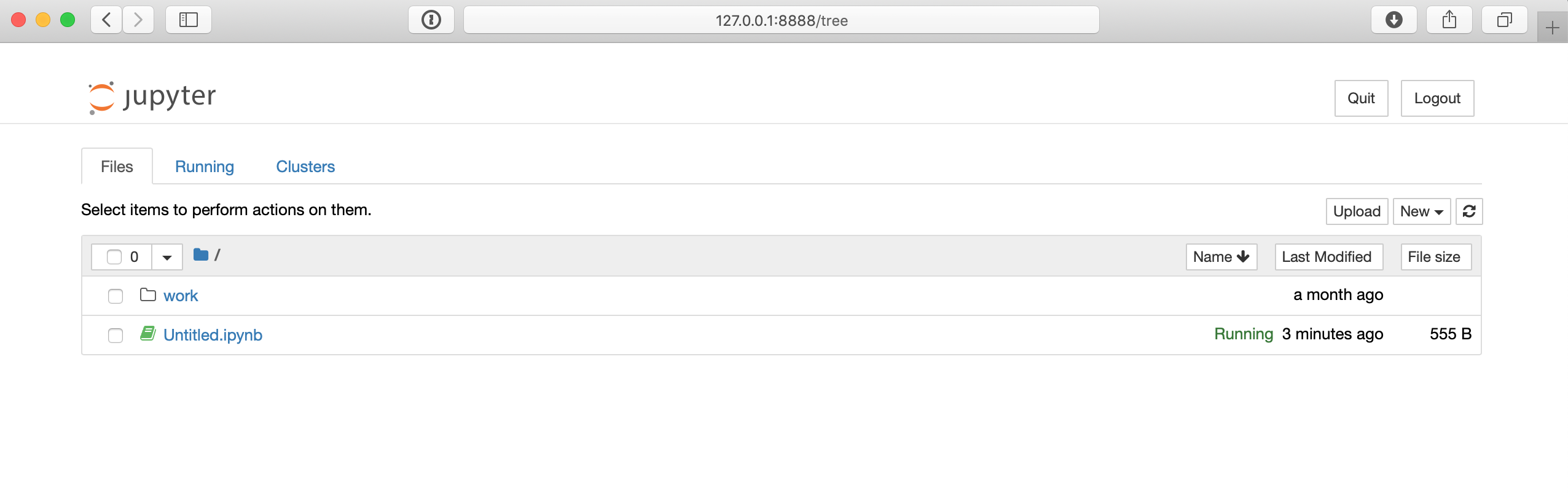
The URL in the command below will likely differ slightly on your machine, but once you connect to that URL in your browser, you can access a Jupyter notebook environment, which should look similar to this:
![Jupyter notebook homepage]()
From the Jupyter notebook page, you can use the New button on the far right to create a new Python 3 shell. Then you can test out some code, like the Hello World example from before:
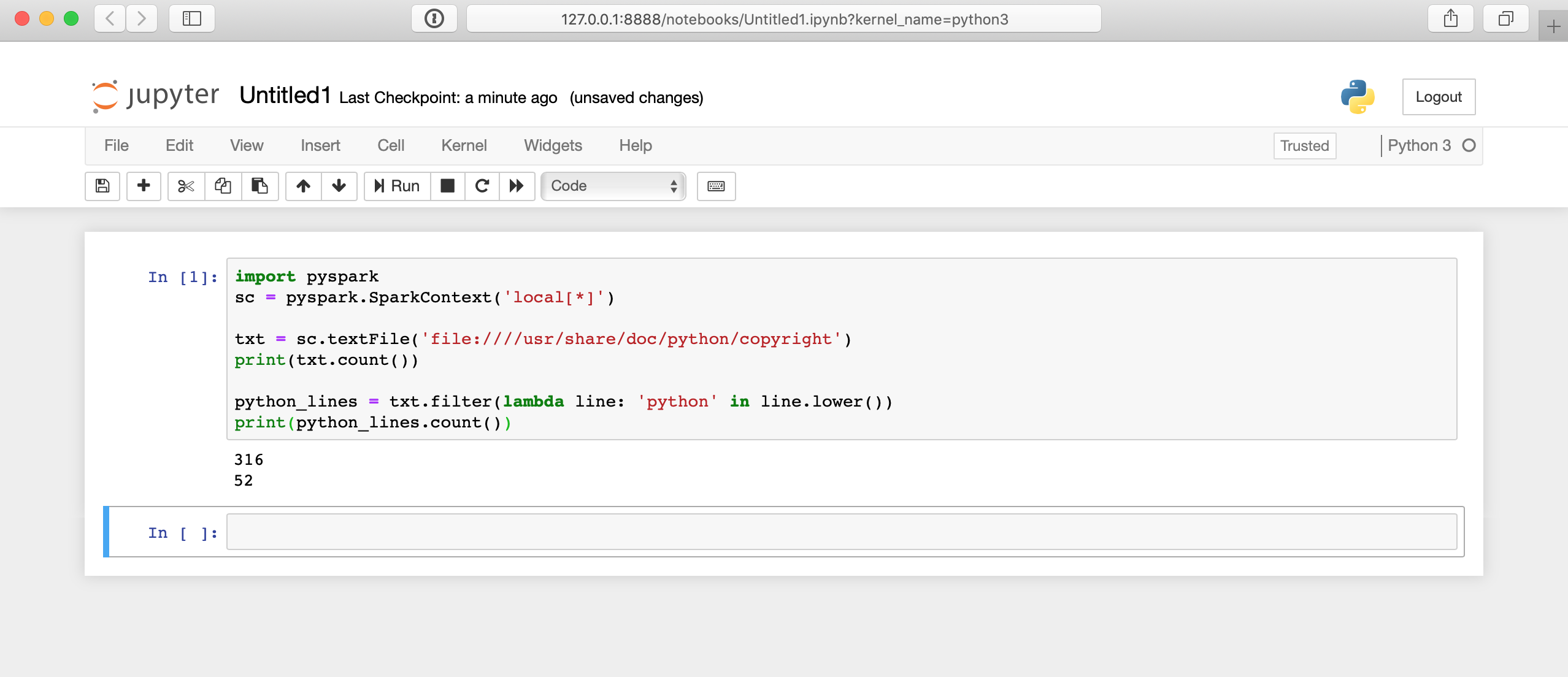
importpysparksc=pyspark.SparkContext('local[*]')txt=sc.textFile('file:////usr/share/doc/python/copyright')print(txt.count())python_lines=txt.filter(lambdaline:'python'inline.lower())print(python_lines.count())Here’s what running that code will look like in the Jupyter notebook:
![PySpark Hello World in Jupyter notebook]()
There is a lot happening behind the scenes here, so it may take a few seconds for your results to display. The answer won’t appear immediately after you click the cell.
Command-Line Interface
The command-line interface offers a variety of ways to submit PySpark programs including the PySpark shell and the spark-submit command. To use these CLI approaches, you’ll first need to connect to the CLI of the system that has PySpark installed.
To connect to the CLI of the Docker setup, you’ll need to start the container like before and then attach to that container. Again, to start the container, you can run the following command:
$ docker run -p 8888:8888 jupyter/pyspark-notebook
Once you have the Docker container running, you need to connect to it via the shell instead of a Jupyter notebook. To do this, run the following command to find the container name:
$ docker container ls
CONTAINER ID        IMAGE                      COMMAND                  CREATED             STATUS              PORTS                    NAMES4d5ab7a93902        jupyter/pyspark-notebook   "tini -g -- start-no…"   12 seconds ago      Up 10 seconds       0.0.0.0:8888->8888/tcp   kind_edison
This command will show you all the running containers. Find the CONTAINER ID of the container running the jupyter/pyspark-notebook image and use it to connect to the bash shell inside the container:
$ docker exec -it 4d5ab7a93902 bash
jovyan@4d5ab7a93902:~$
Now you should be connected to a bash prompt inside of the container. You can verify that things are working because the prompt of your shell will change to be something similar to jovyan@4d5ab7a93902, but using the unique ID of your container.
Note: Replace 4d5ab7a93902 with the CONTAINER ID used on your machine.
Cluster
You can use the spark-submit command installed along with Spark to submit PySpark code to a cluster using the command line. This command takes a PySpark or Scala program and executes it on a cluster. This is likely how you’ll execute your real Big Data processing jobs.
Note: The path to these commands depends on where Spark was installed and will likely only work when using the referenced Docker container.
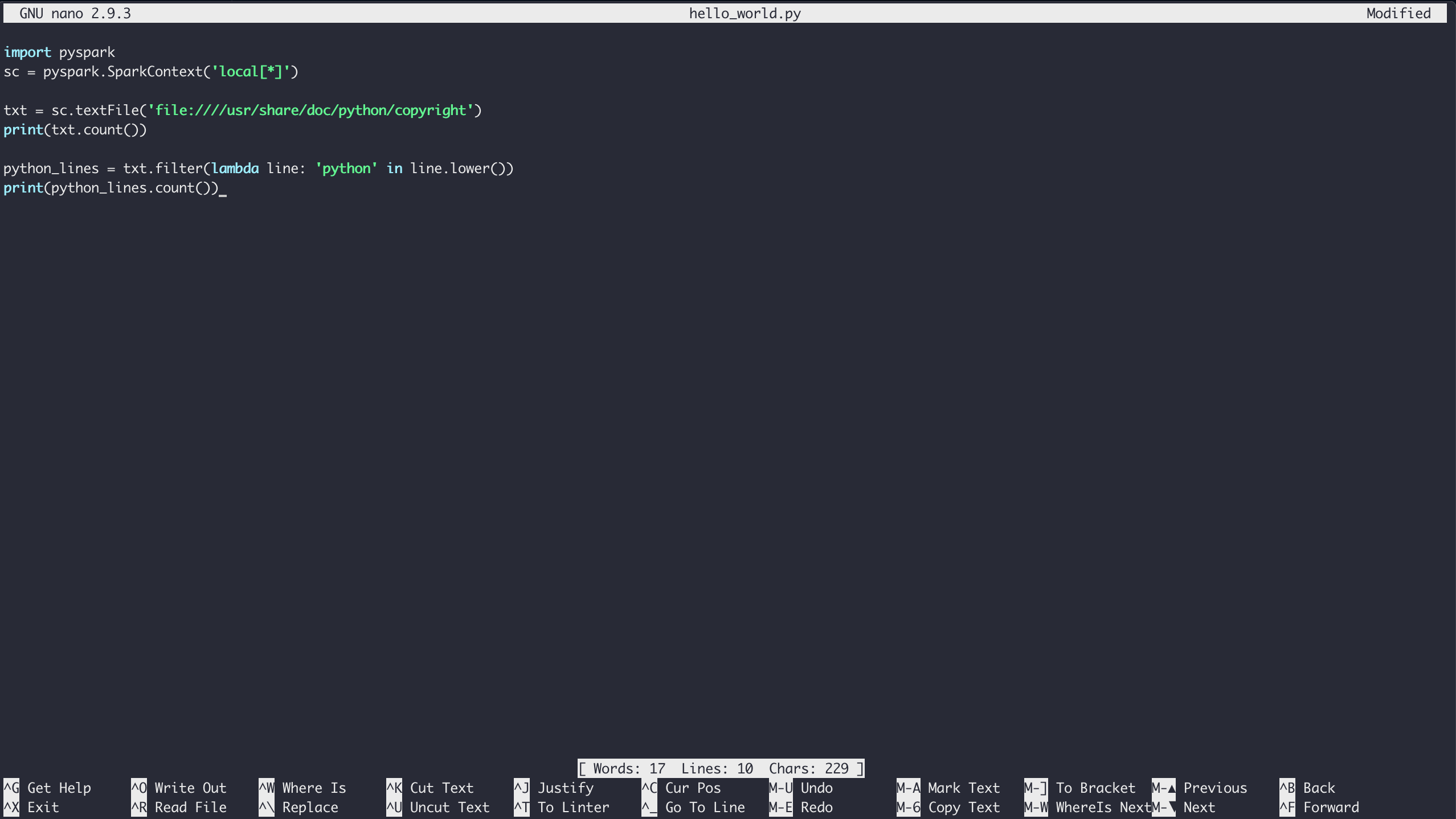
To run the Hello World example (or any PySpark program) with the running Docker container, first access the shell as described above. Once you’re in the container’s shell environment you can create files using the nano text editor.
To create the file in your current folder, simply launch nano with the name of the file you want to create:
Type in the contents of the Hello World example and save the file by typing Ctrl+X and following the save prompts:
![Example using Nano Text Editor]()
Finally, you can run the code through Spark with the pyspark-submit command:
$ /usr/local/spark/bin/spark-submit hello_world.py
This command results in a lot of output by default so it may be difficult to see your program’s output. You can control the log verbosity somewhat inside your PySpark program by changing the level on your SparkContext variable. To do that, put this line near the top of your script:
This will omit some of the output of spark-submit so you can more clearly see the output of your program. However, in a real-world scenario, you’ll want to put any output into a file, database, or some other storage mechanism for easier debugging later.
Luckily, a PySpark program still has access to all of Python’s standard library, so saving your results to a file is not an issue:
importpysparksc=pyspark.SparkContext('local[*]')txt=sc.textFile('file:////usr/share/doc/python/copyright')python_lines=txt.filter(lambdaline:'python'inline.lower())withopen('results.txt','w')asfile_obj:file_obj.write(f'Number of lines: {txt.count()}\n')file_obj.write(f'Number of lines with python: {python_lines.count()}\n')Now your results are in a separate file called results.txt for easier reference later.
Note: The above code uses f-strings, which were introduced in Python 3.6.
PySpark Shell
Another PySpark-specific way to run your programs is using the shell provided with PySpark itself. Again, using the Docker setup, you can connect to the container’s CLI as described above. Then, you can run the specialized Python shell with the following command:
$ /usr/local/spark/bin/pyspark
Python 3.7.3 | packaged by conda-forge | (default, Mar 27 2019, 23:01:00)[GCC 7.3.0] :: Anaconda, Inc. on linuxType "help", "copyright", "credits" or "license" for more information.Using Spark's default log4j profile: org/apache/spark/log4j-defaults.propertiesSetting default log level to "WARN".To adjust logging level use sc.setLogLevel(newLevel). For SparkR, use setLogLevel(newLevel).Welcome to      ____              __     / __/__  ___ _____/ /__    _\ \/ _ \/ _ `/ __/  '_/   /__ / .__/\_,_/_/ /_/\_\   version 2.4.1      /_/Using Python version 3.7.3 (default, Mar 27 2019 23:01:00)SparkSession available as 'spark'.
Now you’re in the Pyspark shell environment inside your Docker container, and you can test out code similar to the Jupyter notebook example:
>>>>>> txt=sc.textFile('file:////usr/share/doc/python/copyright')>>> print(txt.count())316 Now you can work in the Pyspark shell just as you would with your normal Python shell.
Note: You didn’t have to create a SparkContext variable in the Pyspark shell example. The PySpark shell automatically creates a variable, sc, to connect you to the Spark engine in single-node mode.
You must create your ownSparkContext when submitting real PySpark programs with spark-submit or a Jupyter notebook.
You can also use the standard Python shell to execute your programs as long as PySpark is installed into that Python environment. The Docker container you’ve been using does not have PySpark enabled for the standard Python environment. So, you must use one of the previous methods to use PySpark in the Docker container.
As you already saw, PySpark comes with additional libraries to do things like machine learning and SQL-like manipulation of large datasets. However, you can also use other common scientific libraries like NumPy and Pandas.
You must install these in the same environment on each cluster node, and then your program can use them as usual. Then, you’re free to use all the familiar idiomatic Pandas tricks you already know.
Remember:Pandas DataFrames are eagerly evaluated so all the data will need to fit in memory on a single machine.
Next Steps for Real Big Data Processing
Soon after learning the PySpark basics, you’ll surely want to start analyzing huge amounts of data that likely won’t work when you’re using single-machine mode. Installing and maintaining a Spark cluster is way outside the scope of this guide and is likely a full-time job in itself.
So, it might be time to visit the IT department at your office or look into a hosted Spark cluster solution. One potential hosted solution is Databricks.
Databricks allows you to host your data with Microsoft Azure or AWS and has a free 14-day trial.
After you have a working Spark cluster, you’ll want to get all your data into
that cluster for analysis. Spark has a number of ways to import data:
- Amazon S3
- Apache Hive Data Warehouse
- Any database with a JDBC or ODBC interface
You can even read data directly from a Network File System, which is how the previous examples worked.
There’s no shortage of ways to get access to all your data, whether you’re using a hosted solution like Databricks or your own cluster of machines.
Conclusion
PySpark is a good entry-point into Big Data Processing.
In this tutorial, you learned that you don’t have to spend a lot of time learning up-front if you’re familiar with a few functional programming concepts like map(), filter(), and basic Python. In fact, you can use all the Python you already know including familiar tools like NumPy and Pandas directly in your PySpark programs.
You are now able to:
- Understand built-in Python concepts that apply to Big Data
- Write basic PySpark programs
- Run PySpark programs on small datasets with your local machine
- Explore more capable Big Data solutions like a Spark cluster or another custom, hosted solution
[ Improve Your Python With 🐍 Python Tricks 💌 – Get a short & sweet Python Trick delivered to your inbox every couple of days. >> Click here to learn more and see examples ]
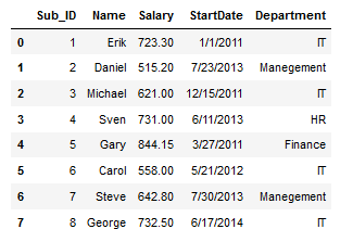
 I was browsing
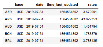
 BTC vs World Currencies table


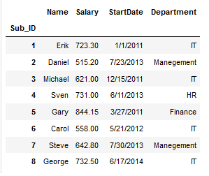
 Python dictionary
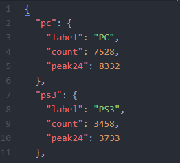
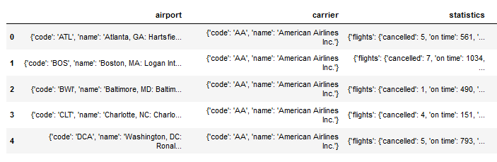 Pandas Dataframe from JSON

 Load the currency symbol from Blockchain