When the data size is not large enough to use distributed computing frameworks (like Apache Spark), processing data in a machine with pandas is an efficient way. But how to insert data with...
↧
Codementor: Graceful Data Ingestion with SQLAlchemy and Pandas
↧
PyCharm: Webinar: “Automating Build, Test and Release Workflows with tox” with Oliver Bestwalter
Python’s tox project is a critical tool for quality software production. Most of our users and customers know about it, but haven’t made the time to learn it.
This webinar’s for you. Oliver Bestwalter is one of the maintainers of tox, and as he discussed in a recent Test and Code interview, has many ideas on how to automate the build/release process.
- Thursday, December 13
- 4:00 PM – 5:00 PM CET (10:00 AM – 11:00 PM EST)
- Register here
- Aimed at intermediate Python developers

Agenda
We will look at what is necessary to automate all important workflows involved in building, testing and releasing software using tox.
We’ll cover how to use tox to …
- run static code analysis, automatic code formatting/fixing as a separate stage orchestrated by the pre-commit framework
- run tests with pytest
- measure and report test coverage
- build and upload packages to pypi/devpi/artifactory
All this can be run and debugged locally from the command line or programmatically.
These building blocks can then form a complete build, test and release pipeline to be run on CI systems like Travis-CI, Gitlab, Jenkins, Teamcity, etc.
If time permits, we’ll also look at how projects like tox and pytest are automating their own processes.
Speaking to You
Oliver is an engineer at Avira who fell in love with open source in the 1990s and with Python in 2006. He creates and helps to maintain test and automation tools helping developers and companies to produce better software more effectively.
Since 2011 he has been a Software Developer at Avira, helping a diverse range of product teams to improve their build, test and release processes. He strives to be a good open source citizen by helping to maintain and improve projects in the area of testing and automation. As part of this effort he spends 20% of his time at Avira working on open source projects. He also enjoys accompanying others on their journey, helping them to improve their skills, and acts as a coach and mentor at Avira and with the Python Academy. When he gets the chance (and can rustle up the courage) he also talks at conferences and meetups.
In 2016 he joined the tox project and is now one of the maintainers. Since 2017 he has been spending up to 20% of his time at Avira working on tox and other open source projects.
-PyCharm Team-
The Drive to Develop
↧
↧
Python Software Foundation: PyPI Security and Accessibility Q1 2019 Request for Proposals period opens.
The Python Software Foundation Packaging Working Group has applied for and received a commitment from the Open Technology Fund to fulfill a contract via their Core Infrastructure Fund.
![]()
![]()
![]()
![]()
![]()
The Python Package Index (PyPI) is a foundational component of the Python ecosystem and broader computer software and technology landscape. This project aims to improve the security and accessibility of PyPI for all users worldwide, whether they are direct users, like project maintainers and
pip installers, or indirect users. The impact of this work will be highly visible and improve crucial features of the service.
We plan to begin the project in January 2019. Because of the size of the project, funding has been allocated to secure one or more contractors to complete the development, testing, verification, and assist in the rollout of necessary features.
Timeline
| Date | Milestone |
|---|---|
| 2018-11-19 | Request for Proposal period opens. |
| 2018-12-14 | Request for Proposal period closes. |
| 2018-12-21 | Date proposals will have received a decision. |
| 2019-Q1 | Contract work commences. |
What is the Request for Proposals period?
A Request for Proposal (RFP) is a process intended to allow us (The Python Software Foundation) to collect proposals from potential contractors and select contractor(s) best suited to fulfill the specified work.
After the RFP period closes we will evaluate the received proposals based on the evaluation criteria, seek clarification from proposers as necessary, and select one or more contractors to complete the work specified in the scope.
The Request for Proposals period opens today, November 19th, 2018, and is scheduled to close December 15, 2018 AoE.
How do I submit a proposal?
First, please read the full contents of the Request for Proposals here!
You'll find the instructions for submission, evaluation criteria, as well as scope of the project there.
↧
Simple is Better Than Complex: Launching our Community Forum
This is a short post just to announce today I’m releasing a community forum for the simpleisbetterthancomplex.com readers! And I want you to be part of it.
I decided to create this community forum for a couple of reasons. First of all, I receive many emails with questions, asking for advice and asking my opinion about specific topics. I’m happy to answer those emails whenever I can, but unfortunately, I can’t answer them all. And when I’m able to answer those emails, the conversations and discussions have a high potential to be useful to others. So why not have some of those discussions in an open forum?
With this community forum, I also want to have a place for questions that are not suitable for StackOverflow. For example, “what’s the best database to use with Django?” or “Apache or NGINX?”. This kind of questions, where there is no right or wrong answer, but can serve as a starting point for a good discussion and exchange of experience.
Another reason is to have a single place to organize the readers’ requests, suggestions, and ideas for future tutorials and videos. There is a specific category for tutorials requests where you can share your ideas and upvote other’s requests to help me prioritize.
And really, I just want this forum to be a safe and respectful place where other tech enthusiasts can get together to talk about tech stuff, share experiences and help each other.
If you want to be part of this community, join us at community.simpleisbetterthancomplex.com!
See you there!
↧
NumFOCUS: NumFOCUS Funds Open Source Projects through Small Development Grants – Fall 2018
The post NumFOCUS Funds Open Source Projects through Small Development Grants – Fall 2018 appeared first on NumFOCUS.
↧
↧
Kushal Das: PyPI and gpg signed packages
Yesterday night, on #pypa IRC channel, asked about uploading detached
gpg signatures for the packages. According to , twine did not upload
the signature, even with passing -s as an argument. I tried to do the same in
test.pypi.org, and at first, I felt the same, as the package
page was not showing anything. As I
started reading the source of twine to figure out what is going on, I found
that it uploads the signature as part of the metadata of package. The JSON
API actually showed that the
release is signed. Later, and explained that we just have
to add .asc at the end of the url of the package to download the detached
signature.
During the conversation, mentioned that only 4% of the total packages are actually gpg signed. And gpg is written in C and also a GPL licensed software, so, it can not be packaged inside of CPython (as pip is packaged inside of CPython). The idea of a future PyPI where all packages must be signed (how will still have to discussed) was also discussed in the IRC channel. We also get to know that we can delete any file/relase from PyPI, but, we can not reload those files again. One has to do a new release. This is also very important incase you want to upload signatures, you will have to do that at the time of uploading the package.
also wrote about the idea of signing the packages a few years ago.
↧
Semaphore Community: Generating Fake Data for Python Unit Tests with Faker
This article is brought with ❤ to you by Semaphore.
Introduction
When writing unit tests, you might come across a situation where you need to generate test data or use some dummy data in your tests. If you already have some data somewhere in a database, one solution you could employ is to generate a dump of that data and use that in your tests (i.e. fixtures).
However, you could also use a package like faker
to generate fake data for you very easily when you need to. This tutorial will
help you learn how to do so in your unit tests.
Prerequisites
For this tutorial, it is expected that you have Python 3.6 and Faker 0.7.11 installed.
Basic Examples in the Command Line
Let's see how this works first by trying out a few things in the shell.
Before we start, go ahead and create a virtual environment and run it:
$ python3 -m venv faker
$ source faker/bin/activate
Once in the environment, install faker.
$ pip install faker
After that, enter the Python REPL by typing the command python in your
terminal.
Once in the Python REPL, start by importing Faker from faker:
Python 3.6.0 (default, Jan  4 2017, 15:38:35)
[GCC 4.2.1 Compatible Apple LLVM 8.0.0 (clang-800.0.42.1)] on darwin
Type "help", "copyright", "credits" or "license" for more information.
>>> from faker import Faker
>>>
Then, we are going to use the Faker class to create a myFactory object whose
methods we will use to generate whatever fake data we need.
>>> myFactory = Faker()
Let's generate a fake text:
>>> myFactory.text()
'Commodi quidem ipsam occaecati. Porro veritatis numquam nisi corrupti.'
As you can see some random text was generated. Yours will probably look very different.
Let us try a few more examples:
>>> myFactory.words()
['libero', 'commodi', 'deleniti']
>>> myFactory.name()
'Joshua Wheeler'
>>> myFactory.month()
'04'
>>> myFactory.sentence()
'Iure expedita eaque at odit soluta repudiandae nam.'
>>> myFactory.state()
'Michigan'
>>> myFactory.random_number()
2950548
You can see how simple the Faker library is to use. Once you have created a factory object, it is very easy to call the provider methods defined on it. You should keep in mind that the output generated on your end will probably be different from what you see in our example — random output.
If you would like to try out some more methods, you can see a list of the
methods you can call on your myFactory object using dir.
>>> dir(myFactory)
You can also find more things to play with in the official docs.
Integrating Faker with an Actual Unit Test
Let's now use what we have learnt in an actual test.
If you are still in the Python REPL, exit by hitting CTRL+D.
Do not exit the virtualenv instance we created and installed Faker to it in
the previous section since we will be using it going forward.
Now, create two files, example.py and test.py, in a folder of your choice.
Our code will live in the example file and our tests in the test file.
Look at this code sample:
# example.pyclassUser:def__init__(self,first_name,last_name,job,address):self.first_name=first_nameself.last_name=last_nameself.job=jobself.address=address@propertydefuser_name(self):returnself.first_name+' '+self.last_name@propertydefuser_job(self):returnself.user_name+" is a "+self.job@propertydefuser_address(self):returnself.user_name+" lives at "+self.addressThis code defines a User class which has a constructor which sets attributes
first_name, last_name, job and address upon object creation.
It also defines class properties user_name, user_job and user_address
which we can use to get a particular user object's properties.
In our test cases, we can easily use Faker to generate all the required data when creating test user objects.
# test.pyimportunittestfromfakerimportFakerfromexampleimportUserclassTestUser(unittest.TestCase):defsetUp(self):self.fake=Faker()self.user=User(first_name=self.fake.first_name(),last_name=self.fake.last_name(),job=self.fake.job(),address=self.fake.address())deftest_user_creation(self):self.assertIsInstance(self.user,User)deftest_user_name(self):expected_username=self.user.first_name+""+self.user.last_nameself.assertEqual(expected_username,self.user.user_name)You can see that we are creating a new User object in the setUp function.
Python calls the setUp function before each test case is run so we can be sure
that our user is available in each test case.
The user object is populated with values directly generated by Faker. We do not need to worry about coming up with data to create user objects. Faker automatically does that for us.
We can then go ahead and make assertions on our User object, without worrying about the data generated at all.
You can run the example test case with this command:
$ python -m unittest
At the moment, we have two test cases, one testing that the user object created is actually an instance of the User class and one testing that the user object's username was constructed properly. Try adding a few more assertions.
Localization
Faker comes with a way of returning localized fake data using some built-in providers. Some built-in location providers include English (United States), Japanese, Italian, and Russian to name a few.
Let's change our locale to to Russia so that we can generate Russian names:
# example.pyfromfakerimportFactorymyGenerator=Factory.create('ru_RU')print(myGenerator.name())In this case, running this code gives us the following output:
> python example.py
Мельникова Прасковья Андреевна
Providers
Providers are just classes which define the methods we call on Faker objects to generate fake data. In the localization example above, the name method we called on the myGenerator object is defined in a provider somewhere. You can see the default included providers here.
Let's create our own provider to test this out.
# example.pyimportrandomfromfakerimportFakerfromfaker.providersimportBaseProviderfake=Faker()# Our custom provider inherits from the BaseProviderclassTravelProvider(BaseProvider):defdestination(self):destinations=['NY','CO','CA','TX','RI']# We select a random destination from the list and return itreturnrandom.choice(destinations)# Add the TravelProvider to our faker objectfake.add_provider(TravelProvider)# We can now use the destination method:print(fake.destination())To define a provider, you need to create a class that inherits from the BaseProvider. That class can then define as many methods as you want. Our TravelProvider example only has one method but more can be added.
Once your provider is ready, add it to your Faker instance like we have done here:
fake.add_provider(TravelProvider)Here is what happens when we run the above example:
$ python example.py
CA
Of course, you output might differ. Try running the script a couple times more to see what happens.
Seeds
Sometimes, you may want to generate the same fake data output every time your code is run. In that case, you need to seed the fake generator.
You can use any random number as a seed.
Example:
# example.pyfromfakerimportFakermyGenerator=Faker()myGenerator.random.seed(5467)foriinrange(10):print(myGenerator.name())Running this code twice generates the same 10 random names:
> python example.py
Denise Reed
Megan Douglas
Philip Obrien
William Howell
Michael Williamson
Cheryl Jackson
Janet Bruce
Colton Martin
David Melton
Paula Ingram
> python example.py
Denise Reed
Megan Douglas
Philip Obrien
William Howell
Michael Williamson
Cheryl Jackson
Janet Bruce
Colton Martin
David Melton
Paula Ingram
If you want to change the output to a different set of random output, you can change the seed given to the generator.
Using Faker on Semaphore
To use Faker on Semaphore, make sure that your project has a requirements.txt file which has faker listed as a dependency.
If you used pip to install Faker, you can easily generate the requirements.txt file by running
the command pip freeze > requirements.txt. This will output a list of all the dependencies installed in your virtualenv
and their respective version numbers into a requirements.txt file.
After pushing your code to git, you can add the project to Semaphore, and then configure your build settings to install Faker
and any other dependencies by running pip install -r requirements.txt. That command simply tells Semaphore to read the
requirements.txt file and add whatever dependencies it defines into the test environment.
After that, executing your tests will be straightforward by using python -m unittest discover.
Conclusion
In this tutorial, you have learnt how to use Faker's built-in providers to generate fake data for your tests, how to use the included location providers to change your locale, and even how to write your own providers.
We also covered how to seed the generator to generate a particular fake data set every time your code is run.
Lastly, we covered how to use Semaphore's platform for Continuous Integration.
Feel free to leave any comments or questions you might have in the comment section below.
This article is brought with ❤ to you by Semaphore.
↧
Chris Moffitt: Building a Repeatable Data Analysis Process with Jupyter Notebooks
Introduction
Over the past couple of months, there has been an ongoing discussion about Jupyter Notebooks affectionately called the “Notebook Wars”. The genesis of the discussion is Joel Grus’ presentation I Don’t Like Notebooks and has been followed up with Tim Hopper’s response, aptly titled I Like Notebooks. There have been several follow-on posts on this topic including thoughtful analysis from Yihui Xie.
The purpose of this post is to use some of the points brought up in these discussions as a background for describing my personal best practices for the analysis I frequently perform with notebooks. In addition, this approach can be tailored for your unique situation. I think many new python users do not take the time to think through some of these items I discuss. My hope is that this article will spark some discussion and provide a framework that others can build off for making repeatable and easy to understand data analysis pipelines that fit their needs.
Specific Use Cases
My use case is much narrower than what Joel describes. As much as possible, I try to use a Jupyter Notebook as my go-to solution when I need to do moderately complex data analysis in a business setting. Instead of creating an Excel spreadsheet, I build a consistent set of notebook files to document my analysis journey. The key distinctions between my approach and the data science scenarios discussed in the presentations above are:
- This analysis is only used by me. I do not share actual python code with anyone. All results are shared by other means (email, presentations, Excel, etc).
- I do not build models that are put into production.
- All analysis is internal, proprietary and not shared publicly.
- If a solution needs to be used by others, I will build a standalone python script for them to use.
- The vast majority of work I describe is data wrangling, EDA and simple statistical analysis. The work is the bread and butter work that Excel is used for in most organizations.
The rest of this article will outline the approach I use in the hopes it can be a framework for others and might help people develop their own repeatable and maintainable work flow.
Why Have Standards?
I imagine that most people that have used Jupyter Notebooks for any significant time have ended up with a directory structure that looks like this:

At a quick glance, there are a lot of problems with this “structure:”
- Inconsistent or absent naming scheme for notebooks
- Mixture of notebooks, scripts, Excel, CSV, images, etc all in one directory
- Vague directory names
- Difficult to follow “flow” of the processing steps
On top of the non-intuitive structure, each notebook has its own unique structure for analyzing data. Some are documented but many are not. None of these issues is a flaw with notebooks per se but is an example of a sloppy approach to solving a problem. You could just as easily end up with this situation with Excel files or stand alone python scripts.
I’ve certainly done all of the things described above. It is incredibly frustrating when I know I did some really useful analysis but I can’t find it 6 months after the fact. If only I had a little more discipline up front, it would have saved a lot of time over the long run.
One of my biggest complaints about Excel is that it is really difficult to understand how the data was pulled together and how all the cells, formulas and VBA relate to each other. There are very limited options for documenting Excel data analysis flow. I believe that using a well-formed Jupyter Notebook structure can lead to a much more reusable set of data analysis artifacts.
Directory Structures
The first step in the process is creating a consistent directory structure. I have leveraged very heavily from the Cookiecutter Data Science project. If you are doing more complex modeling and sharing code with others, then I encourage you to use the above mentioned cookiecutter framework.
In general, I create a new directory for each analysis and take the time to give the directory a descriptive name. Then, I setup the following directory structure:
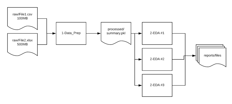
FY_18_Sales_Comp/
  ├── 1-Data_Prep.ipynb
  ├── 2-EDA.ipynb
  ├── data
  │   ├── interim
  │   ├── processed
  │   └── raw
  └── reports
I will cover the details of the notebooks in a bit but the important item to note
is that I include a number followed by the stage in the analysis process. This convention
helps me quickly figure out where I need to go to learn more. If I’m just interested in
the final analysis, I look in the
2-EDA
notebook. If I need to see where the data
comes from, I can jump into
1-Data_Prep
. I will often create multiple EDA files as I
am working through the analysis and try to be as careful as possible about the naming
structure so I can see how items are related.
The other key structural issue is that the input and output files are stored in different directories:
raw- Contains the unedited csv and Excel files used as the source for analysis.interim- Used if there is a multi-step manipulation. This is a scratch location and not always needed but helpful to have in place so directories do not get cluttered or as a temp location form troubleshooting issues.processed- In many cases, I read in multiple files, clean them up and save them to a new location in a binary format. This streamlined format makes it easier to read in larger files later in the processing pipeline.
Finally, any Excel, csv or image output files are stored in the
reports
directory.
Here is a simple diagram of how the data typically flows in these types of scenarios:
Notebook Structure
Once I create each notebook, I try to follow consistent processes for describing the notebooks. The key point to keep in mind is that this header is the first thing you will see when you are trying to figure out how the notebook was used. Trust me, future you will be eternally thankful if you take the time to put some of these comments in the notebook!
Here’s an image of the top of an example notebook:
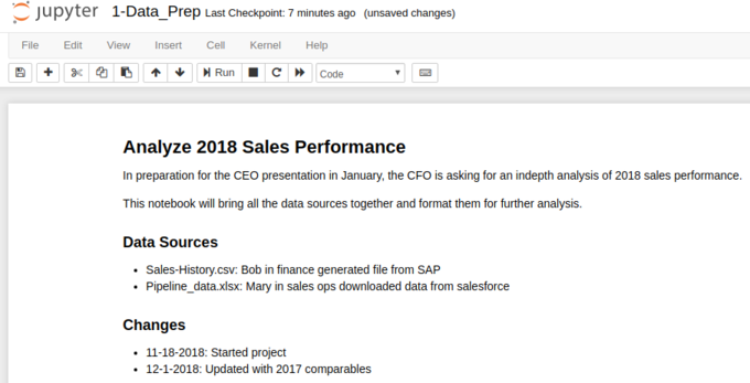
There are a couple of points I always try to include:
- A good name for the notebook (as described above)
- A summary header that describes the project
- Free form description of the business reason for this notebook. I like to include names, dates and snippets of emails to make sure I remember the context.
- A list of people/systems where the data originated.
- I include a simple change log. I find it helpful to record when I started and any major changes along the way. I do not update it with every single change but having some date history is very beneficial.
I tend to include similar imports in most of my notebooks:
importpandasaspdfrompathlibimportPathfromdatetimeimportdatetimeThen I define all my input and output file paths and directories. It is very useful to
do this all in one place at the top of the file. The other key thing I try to do
is make all of my file path references relative to the notebook directory. By
using
Path.cwd()
I can move notebook directories around and it will still work.
I also like to include date and time stamps in the file names. The new f-strings plus pathlib make this simple:
today=datetime.today()sales_file=Path.cwd()/"data"/"raw"/"Sales-History.csv"pipeline_file=Path.cwd()/"data"/"raw"/"pipeline_data.xlsx"summary_file=Path.cwd()/"data"/"processed"/f"summary_{today:%b-%d-%Y}.pkl"If you are not familiar with the Path object, my previous article might be useful.
The other important item to keep in mind is that raw files should NEVER be modified.
The next section of most of my notebooks includes a section to clean up column names. My most common steps are:
- Remove leading and trailing spaces in column names
- Align on a naming convention (dunder, CamelCase, etc.) and stick with it
- When renaming columns, do not include dashes or spaces in names
- Use a rename dictionary to put all the renaming options in one place
- Align on a name for the same value. Account Num, Num, Account ID might all be the same. Name them that way!
- Abbreviations may be ok but make sure it is consistent (for example - always use num vs number)
After cleaning up the columns, I make sure all the data is in the type I expect/need. This previous article on data types should be helpful:
- If you have a need for a date column, make sure it is stored as one.
- Numbers should be
intorfloatand notobject - Categorical types can be used based on your discretion
- If it is a Yes/No, True/False or 1/0 field make sure it is a
boolean - Some data like US zip codes or customer numbers might come in with a leading 0.
If you need to preserve the leading 0, then use an
objecttype.
Once the column names are cleaned up and the data types are correct, I will do the manipulation of the data to get it in the format I need for further analysis.
Here are a few other guidelines to keep in mind:
If you find a particular tricky piece of code that you want to include, be sure to keep a link to where you found it in the notebook.
When saving files to Excel, I like to create an
ExcelWriterobject so I can easily save multiple sheets to the output file. Here is what it looks like:writer=pd.ExcelWriter(report_file,engine='xlsxwriter')df.to_excel(writer,sheet_name='Report')writer.save()
Operationalizing & Customing This Approach
There are a lot of items highlighted here to keep in mind. I am hopeful that readers have thought of their own ideas as well. Fortunately, you can build a simple framework that is easy to replicate for your own analysis by using the cookiecutter project to build your own template. I have placed an example based on this project on github.
Once you install cookiecutter, you can replicate this structure for your own projects:
$ cookiecutter https://github.com/chris1610/pbp_cookiecutter
$ project_name [project_name]: Deep Dive On December Results
$ directory_name [deep_dive_on_december_results]:
$ description [More background on the project]: R&D is trying to understand what happened in December
After answering these questions, you will end up with the directory structure and a sample notebook that looks like this:

The nice result of this approach is that you only need to answer a couple of simple questions to get the template started and populate the notebook with some of the basic project description. My hope is that this lightweight approach will be easy to incorporate into your analysis. I feel this providew a framework for repeatable analysis but is not so burdensome that you do not want to use it because of the additional work in implementing it.
In addition, if you find this approach useful, you could tailor it even more
for your own needs by adding conditional logic to the process or capturing additional
information to include in the notebooks. One idea I have played around with is
including a
snippets.py
file in the cookiecutter template where I save some of
my random/useful code that I use frequently.
I’ll be curious what others think about this approach and any ideas you may have incorporated in your own workflow. Feel free to chime in below with your input in the comments below.
↧
gamingdirectional: Create the Overlap class for Pygame project
Hello there, sorry for a little bit late today because I am busy setting up my old website which is now ready for me to add in more articles into it, if you are interested in more programming articles then do visit this site because I am going to create a brand new laptop application project with python and if you are a python lover then go ahead and bookmark this site and visit it starting from...
Related posts:
 Journey into PyGame — The beginningPygame loads image and background graphic on game sceneThe modify version of the Pygame Missile Manager ClassHow to create a stand still sprite animation with PygameThe most advance sprites overlapping detection method from PygameCreate a Vector class in PygameThe cloud object has been introduced into Rock SweeperPygame Music player demoHow to draw circle with PygameCreate the World module for Rock Sweeper
↧
↧
Mike Driscoll: Python 101: Episode #34 – The SQLAlchemy Package
In this screencast, we learn about the popular SQLAlchemy package. SQLAlchemy is an Object Relational Mapper for Python that allows you to interface with databases in a “Pythonic” manner.
You can also read the chapter this video is based on here or get the book on Leanpub

Note: This video was recorded a couple of years ago, so there may be some minor API changes in SQLAlchemy.
↧
Codementor: NAIMbot - Aim assistant based on machine learning
NAIMbot - Aim assistant based on machine learning
↧
James Bennett: Core no more
If you’re not the sort of person who closely follows the internals of Django’s development, you might not know there’s a draft proposal to drastically change the project’s governance. It’s been getting discussion on GitHub and mailing lists, but I want to take some time today to walk through and explain what this proposal does and what problems it’s trying to solve. So. Let’s dive in.
What’s wrong with Django?
Django the web framework is doing pretty ...
↧
PyCoder’s Weekly: Issue #343 (Nov. 20, 2018)
CPython Governance after Guido, "Clean Architecture" examples, and more
body,#bodyTable,#bodyCell{
height:100% !important;
margin:0;
padding:0;
width:100% !important;
}
table{
border-collapse:collapse;
}
img,a img{
border:0;
outline:none;
text-decoration:none;
}
h1,h2,h3,h4,h5,h6{
margin:0;
padding:0;
}
p{
margin:1em 0;
padding:0;
}
a{
word-wrap:break-word;
}
.mcnPreviewText{
display:none !important;
}
.ReadMsgBody{
width:100%;
}
.ExternalClass{
width:100%;
}
.ExternalClass,.ExternalClass p,.ExternalClass span,.ExternalClass font,.ExternalClass td,.ExternalClass div{
line-height:100%;
}
table,td{
mso-table-lspace:0pt;
mso-table-rspace:0pt;
}
#outlook a{
padding:0;
}
img{
-ms-interpolation-mode:bicubic;
}
body,table,td,p,a,li,blockquote{
-ms-text-size-adjust:100%;
-webkit-text-size-adjust:100%;
}
#bodyCell{
padding:0;
}
.mcnImage,.mcnRetinaImage{
vertical-align:bottom;
}
.mcnTextContent img{
height:auto !important;
}
body,#bodyTable{
background-color:#F2F2F2;
}
#bodyCell{
border-top:0;
}
h1{
color:#555 !important;
display:block;
font-family:Helvetica;
font-size:40px;
font-style:normal;
font-weight:bold;
line-height:125%;
letter-spacing:-1px;
margin:0;
text-align:left;
}
h2{
color:#404040 !important;
display:block;
font-family:Helvetica;
font-size:26px;
font-style:normal;
font-weight:bold;
line-height:125%;
letter-spacing:-.75px;
margin:0;
text-align:left;
}
h3{
color:#555 !important;
display:block;
font-family:Helvetica;
font-size:18px;
font-style:normal;
font-weight:bold;
line-height:125%;
letter-spacing:-.5px;
margin:0;
text-align:left;
}
h4{
color:#808080 !important;
display:block;
font-family:Helvetica;
font-size:16px;
font-style:normal;
font-weight:bold;
line-height:125%;
letter-spacing:normal;
margin:0;
text-align:left;
}
#templatePreheader{
background-color:#3399cc;
border-top:0;
border-bottom:0;
}
.preheaderContainer .mcnTextContent,.preheaderContainer .mcnTextContent p{
color:#ffffff;
font-family:Helvetica;
font-size:11px;
line-height:125%;
text-align:left;
}
.preheaderContainer .mcnTextContent a{
color:#ffffff;
font-weight:normal;
text-decoration:underline;
}
#templateHeader{
background-color:#FFFFFF;
border-top:0;
border-bottom:0;
}
.headerContainer .mcnTextContent,.headerContainer .mcnTextContent p{
color:#555;
font-family:Helvetica;
font-size:15px;
line-height:150%;
text-align:left;
}
.headerContainer .mcnTextContent a{
color:#6DC6DD;
font-weight:normal;
text-decoration:underline;
}
#templateBody{
background-color:#FFFFFF;
border-top:0;
border-bottom:0;
}
.bodyContainer .mcnTextContent,.bodyContainer .mcnTextContent p{
color:#555;
font-size:16px;
line-height:150%;
text-align:left;
margin: 0 0 1em 0;
}
.bodyContainer .mcnTextContent a{
color:#6DC6DD;
font-weight:normal;
text-decoration:underline;
}
#templateFooter{
background-color:#F2F2F2;
border-top:0;
border-bottom:0;
}
.footerContainer .mcnTextContent,.footerContainer .mcnTextContent p{
color:#555;
font-family:Helvetica;
font-size:11px;
line-height:125%;
text-align:left;
}
.footerContainer .mcnTextContent a{
color:#555;
font-weight:normal;
text-decoration:underline;
}
@media only screen and (max-width: 480px){
body,table,td,p,a,li,blockquote{
-webkit-text-size-adjust:none !important;
}
} @media only screen and (max-width: 480px){
body{
width:100% !important;
min-width:100% !important;
}
} @media only screen and (max-width: 480px){
.mcnRetinaImage{
max-width:100% !important;
}
} @media only screen and (max-width: 480px){
table[class=mcnTextContentContainer]{
width:100% !important;
}
} @media only screen and (max-width: 480px){
.mcnBoxedTextContentContainer{
max-width:100% !important;
min-width:100% !important;
width:100% !important;
}
} @media only screen and (max-width: 480px){
table[class=mcpreview-image-uploader]{
width:100% !important;
display:none !important;
}
} @media only screen and (max-width: 480px){
img[class=mcnImage]{
width:100% !important;
}
} @media only screen and (max-width: 480px){
table[class=mcnImageGroupContentContainer]{
width:100% !important;
}
} @media only screen and (max-width: 480px){
td[class=mcnImageGroupContent]{
padding:9px !important;
}
} @media only screen and (max-width: 480px){
td[class=mcnImageGroupBlockInner]{
padding-bottom:0 !important;
padding-top:0 !important;
}
} @media only screen and (max-width: 480px){
tbody[class=mcnImageGroupBlockOuter]{
padding-bottom:9px !important;
padding-top:9px !important;
}
} @media only screen and (max-width: 480px){
table[class=mcnCaptionTopContent],table[class=mcnCaptionBottomContent]{
width:100% !important;
}
} @media only screen and (max-width: 480px){
table[class=mcnCaptionLeftTextContentContainer],table[class=mcnCaptionRightTextContentContainer],table[class=mcnCaptionLeftImageContentContainer],table[class=mcnCaptionRightImageContentContainer],table[class=mcnImageCardLeftTextContentContainer],table[class=mcnImageCardRightTextContentContainer],.mcnImageCardLeftImageContentContainer,.mcnImageCardRightImageContentContainer{
width:100% !important;
}
} @media only screen and (max-width: 480px){
td[class=mcnImageCardLeftImageContent],td[class=mcnImageCardRightImageContent]{
padding-right:18px !important;
padding-left:18px !important;
padding-bottom:0 !important;
}
} @media only screen and (max-width: 480px){
td[class=mcnImageCardBottomImageContent]{
padding-bottom:9px !important;
}
} @media only screen and (max-width: 480px){
td[class=mcnImageCardTopImageContent]{
padding-top:18px !important;
}
} @media only screen and (max-width: 480px){
table[class=mcnCaptionLeftContentOuter] td[class=mcnTextContent],table[class=mcnCaptionRightContentOuter] td[class=mcnTextContent]{
padding-top:9px !important;
}
} @media only screen and (max-width: 480px){
td[class=mcnCaptionBlockInner] table[class=mcnCaptionTopContent]:last-child td[class=mcnTextContent],.mcnImageCardTopImageContent,.mcnCaptionBottomContent:last-child .mcnCaptionBottomImageContent{
padding-top:18px !important;
}
} @media only screen and (max-width: 480px){
td[class=mcnBoxedTextContentColumn]{
padding-left:18px !important;
padding-right:18px !important;
}
} @media only screen and (max-width: 480px){
td[class=mcnTextContent]{
padding-right:18px !important;
padding-left:18px !important;
}
} @media only screen and (max-width: 480px){
table[class=templateContainer]{
max-width:600px !important;
width:100% !important;
}
} @media only screen and (max-width: 480px){
h1{
font-size:24px !important;
line-height:125% !important;
}
} @media only screen and (max-width: 480px){
h2{
font-size:20px !important;
line-height:125% !important;
}
} @media only screen and (max-width: 480px){
h3{
font-size:18px !important;
line-height:125% !important;
}
} @media only screen and (max-width: 480px){
h4{
font-size:16px !important;
line-height:125% !important;
}
} @media only screen and (max-width: 480px){
table[class=mcnBoxedTextContentContainer] td[class=mcnTextContent],td[class=mcnBoxedTextContentContainer] td[class=mcnTextContent] p{
font-size:18px !important;
line-height:125% !important;
}
} @media only screen and (max-width: 480px){
table[id=templatePreheader]{
display:block !important;
}
} @media only screen and (max-width: 480px){
td[class=preheaderContainer] td[class=mcnTextContent],td[class=preheaderContainer] td[class=mcnTextContent] p{
font-size:14px !important;
line-height:115% !important;
}
} @media only screen and (max-width: 480px){
td[class=headerContainer] td[class=mcnTextContent],td[class=headerContainer] td[class=mcnTextContent] p{
font-size:18px !important;
line-height:125% !important;
}
} @media only screen and (max-width: 480px){
td[class=bodyContainer] td[class=mcnTextContent],td[class=bodyContainer] td[class=mcnTextContent] p{
font-size:18px !important;
line-height:125% !important;
}
} @media only screen and (max-width: 480px){
td[class=footerContainer] td[class=mcnTextContent],td[class=footerContainer] td[class=mcnTextContent] p{
font-size:14px !important;
line-height:115% !important;
}
} @media only screen and (max-width: 480px){
td[class=footerContainer] a[class=utilityLink]{
display:block !important;
}
}
![alt]()
Comparison of the 7 Python Governance PEPs
| ||||||||||||||||
|
[ Subscribe to 🐍 PyCoder’s Weekly 💌 – Get the best Python news, articles, and tutorials delivered to your inbox once a week >> Click here to learn more ]
↧
↧
PythonClub - A Brazilian collaborative blog about Python: Algoritmos de Ordenação
Fala pessoal, tudo bom?
Nos vídeos abaixo, vamos aprender como implementar alguns dos algoritmos de ordenação usando Python.
Bubble Sort
Como o algoritmo funciona: Como implementar o algoritmo usando Python: https://www.youtube.com/watch?v=Doy64STkwlI.
Como implementar o algoritmo usando Python: https://www.youtube.com/watch?v=B0DFF0fE4rk.
Código do algoritmo
defsort(array):forfinalinrange(len(array),0,-1):exchanging=Falseforcurrentinrange(0,final-1):ifarray[current]>array[current+1]:array[current+1],array[current]=array[current],array[current+1]exchanging=Trueifnotexchanging:breakSelection Sort
Como o algoritmo funciona: Como implementar o algoritmo usando Python: https://www.youtube.com/watch?v=PLvo_Yb_myrNBhIdq8qqtNSDFtnBfsKL2r.
Como implementar o algoritmo usando Python: https://www.youtube.com/watch?v=0ORfCwwhF_I.
Código do algoritmo
defsort(array):forindexinrange(0,len(array)):min_index=indexforrightinrange(index+1,len(array)):ifarray[right]<array[min_index]:min_index=rightarray[index],array[min_index]=array[min_index],array[index]Insertion Sort
Como o algoritmo funciona: Como implementar o algoritmo usando Python: https://www.youtube.com/watch?v=O_E-Lj5HuRU.
Como implementar o algoritmo usando Python: https://www.youtube.com/watch?v=Sy_Z1pqMgko.
Código do algoritmo
defsort(array):forpinrange(0,len(array)):current_element=array[p]whilep>0andarray[p-1]>current_element:array[p]=array[p-1]p-=1array[p]=current_element↧
Vladimir Iakolev: Analysing the trip to South America with a bit of image recognition
Back in September, I had a three weeks trip to South America. While planning the trip I was using sort of data mining to select the most optimal flights and it worked well. To continue following the data-driven approach (more buzzwords), I’ve decided to analyze the data I’ve collected during the trip.
Unfortunately, I was traveling without local sim-card and almost without internet, I can’t use Google Location History as in the fun research about the commute. But at least I have tweets and a lot of photos.
At first, I’ve reused old code(more internal linking) and extracted information about flights from tweets:
all_tweets=pd.DataFrame([(tweet.text,tweet.created_at)fortweetinget_tweets()],# get_tweets available in the gistcolumns=['text','created_at'])tweets_in_dates=all_tweets[(all_tweets.created_at>datetime(2018,9,8))&(all_tweets.created_at<datetime(2018,9,30))]flights_tweets=tweets_in_dates[tweets_in_dates.text.str.upper()==tweets_in_dates.text]flights=flights_tweets.assign(start=lambdadf:df.text.str.split('✈').str[0],finish=lambdadf:df.text.str.split('✈').str[-1]) \
.sort_values('created_at')[['start','finish','created_at']]>>>flightsstartfinishcreated_at19AMS️LIS2018-09-0805:00:3218LIS️GIG2018-09-0811:34:1417SDU️EZE2018-09-1223:29:5216EZE️SCL2018-09-1617:30:0115SCL️LIM2018-09-1916:54:1314LIM️MEX2018-09-2220:43:4213MEX️CUN2018-09-2519:29:0411CUN️MAN2018-09-2920:16:11Then I’ve found a json dump with airports, made a little hack with replacing Ezeiza with Buenos-Aires and found cities with lengths of stay from flights:
flights=flights.assign(start=flights.start.apply(lambdacode:iata_to_city[re.sub(r'\W+','',code)]),# Removes leftovers of emojis, iata_to_city available in the gistfinish=flights.finish.apply(lambdacode:iata_to_city[re.sub(r'\W+','',code)]))cities=flights.assign(spent=flights.created_at-flights.created_at.shift(1),city=flights.start,arrived=flights.created_at.shift(1),)[["city","spent","arrived"]]cities=cities.assign(left=cities.arrived+cities.spent)[cities.spent.dt.days>0]>>>citiescityspentarrivedleft17RioDeJaneiro4days11:55:382018-09-0811:34:142018-09-1223:29:5216Buenos-Aires3days18:00:092018-09-1223:29:522018-09-1617:30:0115Santiago2days23:24:122018-09-1617:30:012018-09-1916:54:1314Lima3days03:49:292018-09-1916:54:132018-09-2220:43:4213MexicoCity2days22:45:222018-09-2220:43:422018-09-2519:29:0411Cancun4days00:47:072018-09-2519:29:042018-09-2920:16:11>>>cities.plot(x="city",y="spent",kind="bar",legend=False,title='Cities') \
.yaxis.set_major_formatter(formatter)# Ugly hack for timedelta formatting, more in the gist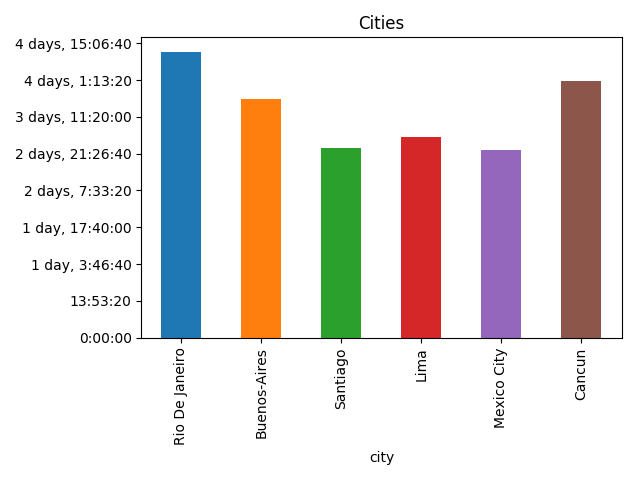
Now it’s time to work with photos. I’ve downloaded all photos from Google Photos, parsed creation dates from Exif, and “joined” them with cities by creation date:
raw_photos=pd.DataFrame(list(read_photos()),columns=['name','created_at'])# read_photos available in the gistphotos_cities=raw_photos.assign(key=0).merge(cities.assign(key=0),how='outer')photos=photos_cities[(photos_cities.created_at>=photos_cities.arrived)&(photos_cities.created_at<=photos_cities.left)]>>>photos.head()namecreated_atkeycityspentarrivedleft1photos/20180913_183207.jpg2018-09-1318:32:070Buenos-Aires3days18:00:092018-09-1223:29:522018-09-1617:30:016photos/20180909_141137.jpg2018-09-0914:11:360RioDeJaneiro4days11:55:382018-09-0811:34:142018-09-1223:29:5214photos/20180917_162240.jpg2018-09-1716:22:400Santiago2days23:24:122018-09-1617:30:012018-09-1916:54:1322photos/20180923_161707.jpg2018-09-2316:17:070MexicoCity2days22:45:222018-09-2220:43:422018-09-2519:29:0426photos/20180917_111251.jpg2018-09-1711:12:510Santiago2days23:24:122018-09-1617:30:012018-09-1916:54:13After that I’ve got the amount of photos by city:
photos_by_city=photos \
    .groupby(by='city') \
    .agg({'name':'count'}) \
    .rename(columns={'name':'photos'}) \
.reset_index()>>>photos_by_citycityphotos0Buenos-Aires1931Cancun2922Lima2953MexicoCity2564RioDeJaneiro4225Santiago267>>>photos_by_city.plot(x='city',y='photos',kind="bar",title='Photos by city',legend=False)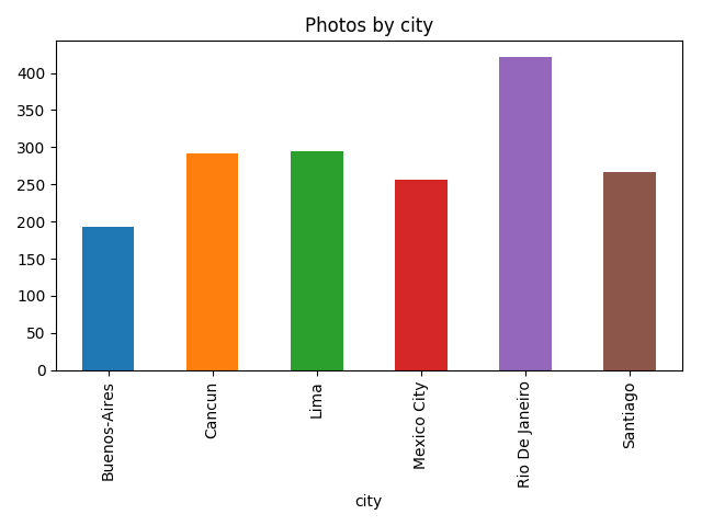
Let’s go a bit deeper and use image recognition, to not reinvent the wheel I’ve used a slightly modified version of TensorFlow imagenet tutorial example and for each photo find what’s on it:
classify_image.init()tags=tagged_photos.name\
    .apply(lambdaname:classify_image.run_inference_on_image(name,1)[0]) \
.apply(pd.Series)tagged_photos=photos.copy()tagged_photos[['tag','score']]=tags.apply(pd.Series)tagged_photos['tag']=tagged_photos.tag.apply(lambdatag:tag.split(', ')[0])>>>tagged_photos.head()namecreated_atkeycityspentarrivedlefttagscore1photos/20180913_183207.jpg2018-09-1318:32:070Buenos-Aires3days18:00:092018-09-1223:29:522018-09-1617:30:01cinema0.1644156photos/20180909_141137.jpg2018-09-0914:11:360RioDeJaneiro4days11:55:382018-09-0811:34:142018-09-1223:29:52pedestal0.66712814photos/20180917_162240.jpg2018-09-1716:22:400Santiago2days23:24:122018-09-1617:30:012018-09-1916:54:13cinema0.22540422photos/20180923_161707.jpg2018-09-2316:17:070MexicoCity2days22:45:222018-09-2220:43:422018-09-2519:29:04obelisk0.77524426photos/20180917_111251.jpg2018-09-1711:12:510Santiago2days23:24:122018-09-1617:30:012018-09-1916:54:13seashore0.24720So now it’s possible to find things that I’ve taken photos of the most:
photos_by_tag=tagged_photos \
    .groupby(by='tag') \
    .agg({'name':'count'}) \
    .rename(columns={'name':'photos'}) \
    .reset_index() \
    .sort_values('photos',ascending=False) \
.head(10)>>>photos_by_tagtagphotos107seashore27676monastery14264lakeside11686palace1153alp8681obelisk72101promontory50105sandbar4917bellcote4339cliff42>>>photos_by_tag.plot(x='tag',y='photos',kind='bar',legend=False,title='Popular tags')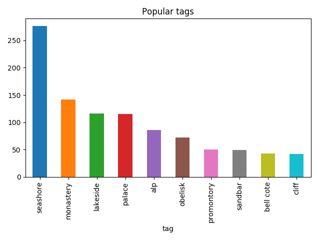
Then I was able to find what I was taking photos of by city:
popular_tags=photos_by_tag.head(5).tagpopular_tagged=tagged_photos[tagged_photos.tag.isin(popular_tags)]not_popular_tagged=tagged_photos[~tagged_photos.tag.isin(popular_tags)].assign(tag='other')by_tag_city=popular_tagged \
    .append(not_popular_tagged) \
    .groupby(by=['city','tag']) \
    .count()['name'] \
.unstack(fill_value=0)>>>by_tag_citytagalplakesidemonasteryotherpalaceseashorecityBuenos-Aires51241233010Cancun01961534110Lima025421363854MexicoCity7926197512RioDeJaneiro734517212471Santiago117271693419>>>by_tag_city.plot(kind='bar',stacked=True)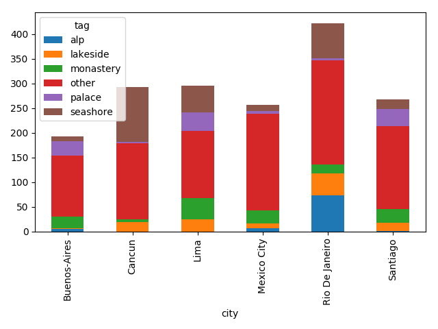
Although the most common thing on this plot is “other”, it’s still fun.
↧
Talk Python to Me: #187 Secure all the things with HubbleStack
How do you keep track of the security, configuration states, and even out of date system level packages in your servers? What if you had 40,000 or more servers? How's your process scale? I'll tell you, mine would take some tweaks!
↧
Mike Driscoll: Black Friday / Cyber Monday Sale 2018
This week I am putting my 2 most recent self-published books on Sale starting today through November 26th.

ReportLab – PDF Processing with Python is available for $9.99:

JupyterLab 101 is available for $9.99:

You can also get my book, wxPython Recipes, from Apress for $7 for a limited time with the following coupon code: cyberweek18.

Python Interviews is $10 right now too!
↧
↧
gamingdirectional: Create a pool object for enemy ships
In this article we will start to create a pool object which will recycle the enemy ship and then we will create a new object pool for the missiles on the next article. Before we can create a pool object we will need to create the Objectpool class first which has two important methods:- 1) Put the enemy ship to an object pool when it gets removed by the enemy list. 2) Return the ship again to the...
Related posts:
Pygame tutorial 2 – Moving the object with keyboardCreate player missile manager and player missile class in PygamePygame’s Color class demoCreate the spaceship in Rock SweeperGroup all the sprites together with PygameHow to move and flip the gaming character with PygamePlaying background music with PygameMoving the sprite with Vector in PygameHow to detect boundary in PygameCreate Enemy Missile and Enemy Missile Manager↧
Real Python: Memory Management in Python
Ever wonder how Python handles your data behind the scenes? How are your variables stored in memory? When do they get deleted?
In this article, we’re going to do a deep dive into the internals of Python to understand how it handles memory management.
By the end of this article, you’ll:
- Learn more about low-level computing, specifically as relates to memory
- Understand how Python abstracts lower-level operations
- Learn about Python’s internal memory management algorithms
Understanding Python’s internals will also give you better insight into some of Python’s behaviors. Hopefully, you’ll gain a new appreciation for Python as well. So much logic is happening behind the scenes to ensure your program works the way you expect.
Free Bonus:5 Thoughts On Python Mastery, a free course for Python developers that shows you the roadmap and the mindset you'll need to take your Python skills to the next level.
Memory Is an Empty Book
You can begin by thinking of a computer’s memory as an empty book intended for short stories. There’s nothing written on the pages yet. Eventually, different authors will come along. Each author wants some space to write their story in.
Since they aren’t allowed to write over each other, they must be careful about which pages they write in. Before they begin writing, they consult the manager of the book. The manager then decides where in the book they’re allowed to write.
Since this book is around for a long time, many of the stories in it are no longer relevant. When no one reads or references the stories, they are removed to make room for new stories.
In essence, computer memory is like that empty book. In fact, it’s common to call fixed-length contiguous blocks of memory pages, so this analogy holds pretty well.
The authors are like different applications or processes that need to store data in memory. The manager, who decides where the authors can write in the book, plays the role of a memory manager of sorts. The person who removed the old stories to make room for new ones is a garbage collector.
Memory Management: From Hardware to Software
Memory management is the process by which applications read and write data. A memory manager determines where to put an application’s data. Since there’s a finite chunk of memory, like the pages in our book analogy, the manager has to find some free space and provide it to the application. This process of providing memory is generally called memory allocation.
On the flip side, when data is no longer needed, it can be deleted, or freed. But freed to where? Where did this “memory” come from?
Somewhere in your computer, there’s a physical device storing data when you’re running your Python programs. There are many layers of abstraction that the Python code goes through before the objects actually get to the hardware though.
One of the main layers above the hardware (such as RAM or a hard drive) is the operating system (OS). It carries out (or denies) requests to read and write memory.
Above the OS, there are applications, one of which is the default Python implementation (included in your OS or downloaded from python.org). Memory management for your Python code is handled by the Python application. The algorithms and structures that the Python application uses for memory management is the focus of this article.
The Default Python Implementation
The default Python implementation, CPython, is actually written in the C programming language.
When I first heard this, it blew my mind. A language that’s written in another language?! Well, not really, but sort of.
The Python language is defined in a reference manual written in English. However, that manual isn’t all that useful by itself. You still need something to interpret written code based on the rules in the manual.
You also need something to actually execute interpreted code on a computer. The default Python implementation fulfills both of those requirements. It converts your Python code into instructions that it then runs on a virtual machine.
Note: Virtual machines are like physical computers, but they are implemented in software. They typically process basic instructions similar to Assembly instructions.
Python is an interpreted programming language. Your Python code actually gets compiled down to more computer-readable instructions called bytecode. These instructions get interpreted by a virtual machine when you run your code.
Have you ever seen a .pyc file or a __pycache__ folder? That’s the bytecode that gets interpreted by the virtual machine.
It’s important to note that there are implementations other than CPython. IronPython compiles down to run on Microsoft’s Common Language Runtime. Jython compiles down to Java bytecode to run on the Java Virtual Machine. Then there’s PyPy, but that deserves its own entire article, so I’ll just mention it in passing.
For the purposes of this article, I’ll focus on the memory management done by the default implementation of Python, CPython.
Disclaimer: While a lot of this information will carry through to new versions of Python, things may change in the future. Note that the referenced version for this article is the current latest version of Python, 3.7.
Okay, so CPython is written in C, and it interprets Python bytecode. What does this have to do with memory management? Well, the memory management algorithms and structures exist in the CPython code, in C. To understand the memory management of Python, you have to get a basic understanding of CPython itself.
CPython is written in C, which does not natively support object-oriented programming. Because of that, there are quite a bit of interesting designs in the CPython code.
You may have heard that everything in Python is an object, even types such as int and str. Well, it’s true on an implementation level in CPython. There is a struct called a PyObject, which every other object in CPython uses.
Note: A struct, or structure, in C is a custom data type that groups together different data types. To compare to object-oriented languages, it’s like a class with attributes and no methods.
The PyObject, the grand-daddy of all objects in Python, contains only two things:
ob_refcnt: reference countob_type: pointer to another type
The reference count is used for garbage collection. Then you have a pointer to the actual object type. That object type is just another struct that describes a Python object (such as a dict or int).
Each object has its own object-specific memory allocator that knows how to get the memory to store that object. Each object also has an object-specific memory deallocator that “frees” the memory once it’s no longer needed.
However, there’s an important factor in all this talk about allocating and freeing memory. Memory is a shared resource on the computer, and bad things can happen if two different processes try to write to the same location at the same time.
The Global Interpreter Lock (GIL)
The GIL is a solution to the common problem of dealing with shared resources, like memory in a computer. When two threads try to modify the same resource at the same time, they can step on each other’s toes. The end result can be a garbled mess where neither of the threads ends up with what they wanted.
Consider the book analogy again. Suppose that two authors stubbornly decide that it’s their turn to write. Not only that, but they both need to write on the same page of the book at the same time.
They each ignore the other’s attempt to craft a story and begin writing on the page. The end result is two stories on top of each other, which makes the whole page completely unreadable.
One solution to this problem is a single, global lock on the interpreter when a thread is interacting with the shared resource (the page in the book). In other words, only one author can write at a time.
Python’s GIL accomplishes this by locking the entire interpreter, meaning that it’s not possible for another thread to step on the current one. When CPython handles memory, it uses the GIL to ensure that it does so safely.
There are pros and cons to this approach, and the GIL is heavily debated in the Python community. To read more about the GIL, I suggest checking out What is the Python Global Interpreter Lock (GIL)?.
Garbage Collection
Let’s revisit the book analogy and assume that some of the stories in the book are getting very old. No one is reading or referencing those stories anymore. If no one is reading something or referencing it in their own work, you could get rid of it to make room for new writing.
That old, unreferenced writing could be compared to an object in Python whose reference count has dropped to 0. Remember that every object in Python has a reference count and a pointer to a type.
The reference count gets increased for a few different reasons. For example, the reference count will increase if you assign it to another variable:
numbers=[1,2,3]# Reference count = 1more_numbers=numbers# Reference count = 2It will also increase if you pass the object as an argument:
total=sum(numbers)As a final example, the reference count will increase if you include the object in a list:
matrix=[numbers,numbers,numbers]Python allows you to inspect the current reference count of an object with the sys module. You can use sys.getrefcount(numbers), but keep in mind that passing in the object to getrefcount() increases the reference count by 1.
In any case, if the object is still required to hang around in your code, its reference count is greater than 0. Once it drops to 0, the object has a specific deallocation function that is called which “frees” the memory so that other objects can use it.
But what does it mean to “free” the memory, and how do other objects use it? Let’s jump right into CPython’s memory management.
CPython’s Memory Management
We’re going to dive deep into CPython’s memory architecture and algorithms, so buckle up.
As mentioned before, there are layers of abstraction from the physical hardware to CPython. The operating system (OS) abstracts the physical memory and creates a virtual memory layer that applications (including Python) can access.
An OS-specific virtual memory manager carves out a chunk of memory for the Python process. The darker gray boxes in the image below are now owned by the Python process.

Python uses a portion of the memory for internal use and non-object memory. The other portion is dedicated to object storage (your int, dict, and the like). Note that this was somewhat simplified. If you want the full picture, you can check out the CPython source code, where all this memory management happens.
CPython has an object allocator that is responsible for allocating memory within the object memory area. This object allocator is where most of the magic happens. It gets called every time a new object needs space allocated or deleted.
Typically, the adding and removing of data for Python objects like list and int doesn’t involve too much data at a time. So the design of the allocator is tuned to work well with small amounts of data at a time. It also tries not to allocate memory until it’s absolutely required.
The comments in the source code describe the allocator as “a fast, special-purpose memory allocator for small blocks, to be used on top of a general-purpose malloc.” In this case, malloc is C’s library function for memory allocation.
Now we’ll look at CPython’s memory allocation strategy. First, we’ll talk about the 3 main pieces and how they relate to each other.
Arenas are the largest chunks of memory and are aligned on a page boundary in memory. A page boundary is the edge of a fixed-length contiguous chunk of memory that the OS uses. Python assumes the system’s page size is 256 kilobytes.

Within the arenas are pools, which are one virtual memory page (4 kilobytes). These are like the pages in our book analogy. These pools are fragmented into smaller blocks of memory.
All the blocks in a given pool are of the same “size class.” A size class defines a specific block size, given some amount of requested data. The chart below is taken directly from the source code comments:
| Request in bytes | Size of allocated block | Size class idx |
|---|---|---|
| 1-8 | 8 | 0 |
| 9-16 | 16 | 1 |
| 17-24 | 24 | 2 |
| 25-32 | 32 | 3 |
| 33-40 | 40 | 4 |
| 41-48 | 48 | 5 |
| 49-56 | 56 | 6 |
| 57-64 | 64 | 7 |
| 65-72 | 72 | 8 |
| … | … | … |
| 497-504 | 504 | 62 |
| 505-512 | 512 | 63 |
For example, if 42 bytes are requested, the data would be placed into a size 48-byte block.
Pools
Pools are composed of blocks from a single size class. Each pool maintains a double-linked list to other pools of the same size class. In that way, the algorithm can easily find available space for a given block size, even across different pools.
A usedpools list tracks all the pools that have some space available for data for each size class. When a given block size is requested, the algorithm checks this usedpools list for the list of pools for that block size.
Pools themselves must be in one of 3 states: used, full, or empty. A used pool has available blocks for data to be stored. A full pool’s blocks are all allocated and contain data. An empty pool has no data stored and can be assigned any size class for blocks when needed.
A freepools list keeps track of all the pools in the empty state. But when do empty pools get used?
Assume your code needs an 8-byte chunk of memory. If there are no pools in usedpools of the 8-byte size class, a fresh empty pool is initialized to store 8-byte blocks. This new pool then gets added to the usedpools list so it can be used for future requests.
Say a full pool frees some of its blocks because the memory is no longer needed. That pool would get added back to the usedpools list for its size class.
You can see now how pools can move between these states (and even memory size classes) freely with this algorithm.
Blocks
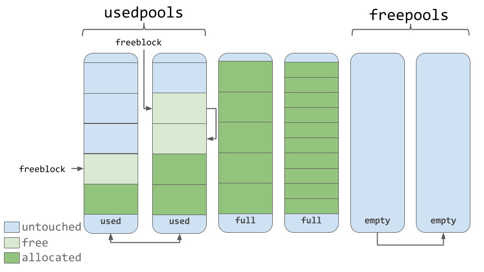
As seen in the diagram above, pools contain a pointer to their “free” blocks of memory. There’s a slight nuance to the way this works. This allocator “strives at all levels (arena, pool, and block) never to touch a piece of memory until it’s actually needed,” according to the comments in the source code.
That means that a pool can have blocks in 3 states. These states can be defined as follows:
untouched: a portion of memory that has not been allocatedfree: a portion of memory that was allocated but later made “free” by CPython and that no longer contains relevant dataallocated: a portion of memory that actually contains relevant data
The freeblock pointer points to a singly linked list of free blocks of memory. In other words, a list of available places to put data. If more than the available free blocks are needed, the allocator will get some untouched blocks in the pool.
As the memory manager makes blocks “free,” those now free blocks get added to the front of the freeblock list. The actual list may not be contiguous blocks of memory, like the first nice diagram. It may look something like the diagram below:

Arenas
Arenas contain pools. Those pools can be used, full, or empty. Arenas themselves don’t have as explicit states as pools do though.
Arenas are instead organized into a doubly linked list called usable_arenas. The list is sorted by the number of free pools available. The fewer free pools, the closer the arena is to the front of the list.

This means that the arena that is the most full of data will be selected to place new data into. But why not the opposite? Why not place data where there’s the most available space?
This brings us to the idea of truly freeing memory. You’ll notice that I’ve been saying “free” in quotes quite a bit. The reason is that when a block is deemed “free”, that memory is not actually freed back to the operating system. The Python process keeps it allocated and will use it later for new data. Truly freeing memory returns it to the operating system to use.
Arenas are the only things that can truly be freed. So, it stands to reason that those arenas that are closer to being empty should be allowed to become empty. That way, that chunk of memory can be truly freed, reducing the overall memory footprint of your Python program.
Conclusion
Memory management is an integral part of working with computers. Python handles nearly all of it behind the scenes, for better or for worse.
In this article, you learned:
- What memory management is and why it’s important
- How the default Python implementation, CPython, is written in the C programming language
- How the data structures and algorithms work together in CPython’s memory management to handle your data
Python abstracts away a lot of the gritty details of working with computers. This gives you the power to work on a higher level to develop your code without the headache of worrying about how and where all those bytes are getting stored.
[ Improve Your Python With 🐍 Python Tricks 💌 – Get a short & sweet Python Trick delivered to your inbox every couple of days. >> Click here to learn more and see examples ]
↧
Stack Abuse: Lists vs Tuples in Python
Introduction
Lists and tuples are two of the most commonly used data structures in Python, with dictionary being the third. Lists and tuples have many similarities. Some of them have been enlisted below:
- They are both sequence data types that store a collection of items
- They can store items of any data type
- And any item is accessible via its index.
So the question we're trying to answer here is, how are they different? And if there is no difference between the two, why should we have the two? Can't we have either lists or tuples?
In this article, we will show how lists and tuples differ from each other.
Syntax Difference
In Python, lists and tuples are declared in different ways. A list is created using square brackets [] whereas the tuple is ceated using parenthesis (). Look at the following example:
tuple_names = ('Nicholas', 'Michelle', 'Alex')
list_names = ['Nicholas', 'Michelle', 'Alex']
print(tuple_names)
print(list_names)
Output:
('Nicholas', 'Michelle', 'Alex')
['Nicholas', 'Michelle', 'Alex']
We defined a tuple named tuple_names and a list named list_names. In the tuple definition, we used parenthesis () while in the list definition, we used square brackets [].
Python has the type() object that helps us know the type of an object that has been created. We can use it as follows:
print(type(tuple_names))
print(type(list_names))
Output:
<class 'tuple'>
<class 'list'>
Mutable vs. Immutable
Lists are mutable while tuples are immutable, and this marks the KEY difference between the two. But what do we mean by this?
The answer is this: we can change/modify the values of a list but we cannot change/modify the values of a tuple.
Since lists are mutable, we can't use a list as a key in a dictionary. This is because only an immutable object can be used as a key in a dictionary. Thus, we can use tuples as dictionary keys if needed.
Let's take a look at an example that demonstrates the difference between lists and tuple in terms of immutability.
Let us create a list of differen names:
names = ["Nicholas", "Michelle", "Alex"]
Let us see what will happen if we attempt to change the first element of the list from "Nicholas" to "Samuel":
names[0] = "Samuel"Note that the first element is at index 0.
Now, let us display the contents of the list:
>>> names
Output:
['Samuel', 'Michelle', 'Alex']
The output shows that the first item of the list was changed successfully!
What if we attempt to do the same with a tuple? Let's see:
First, create the tuple:
names = ("Nicholas", "Michelle", "Alex")
Let us now attempt to change the first element of the tuple from "Nicholas" to "Samuel":
names[0] = "Samuel"Output:
Traceback (most recent call last):
  File "<pyshell#7>", line 1, in <module>
    names[0] = "Samuel"
TypeError: 'tuple' object does not support item assignment
We got an error that a tuple object does not support item assignment. The reason is that a tuple object cannot be changed after it has been created.
Reused vs. Copied
Tuples cannot be copied. The reason is that tuples are immutable. If you run tuple(tuple_name), it will immediately return itself. For example:
names = ('Nicholas', 'Michelle', 'Alex')
copyNames = tuple(names)
print(names is copyNames)
Output:
True
The two are the same.
In contrast, list(list_name) requires copying of all data to a new list. For example:
names = ['Nicholas', 'Michelle', 'Alex']
copyNames = list(names)
print(names is copyNames)
Output:
False
Next, let us discuss how the list and the tuple differ in terms of size.
Size Difference
Python allocates memory to tuples in terms of larger blocks with a low overhead because they are immutable. On the other hand, for lists, Pythons allocates small memory blocks. At the end of it, the tuple will have a smaller memory compared to the list. This makes tuples a bit faster than lists when you have a large number of elements.
For example:
tuple_names = ('Nicholas', 'Michelle', 'Alex')
list_names = ['Nicholas', 'Michelle', 'Alex']
print(tuple_names.__sizeof__())
print(list_names.__sizeof__())
Output:
48
64
The above output shows that the list has a larger size than the tuple. The size shown is in terms of bytes.
Homogeneous vs. Heterogeneous
Tuples are used to store heterogeneous elements, which are elements belonging to different data types. Lists, on the other hand, are used to store homogenous elements, which are elements that belong to the same type.
However, note that this is only a semantic difference. You can store elements of the same type in a tuple and elements of different types in a list. For example:
list_elements = ['Nicholas', 10, 'Alex']
tuple_elements = ('Nicholas', "Michelle", 'Alex')
The above code will run with no error despite the fact that the list has a mixture of strings and a number.
Variable Length vs. Fixed Length
Tuples have a fixed length while lists have a variable length. This means we can change the size of a created list but we cannot change the size of an existing tuple. For example:
list_names = ['Nicholas', 'Michelle', 'Alex']
list_names.append("Mercy")
print(list_names)
Output:
['Nicholas', 'Michelle', 'Alex', 'Mercy']
The output shows that a fourth name has been added to the list. We have used the Python's append() function for this. We could have achieved the same via the insert() function as shown below:
list_names = ['Nicholas', 'Michelle', 'Alex']
list_names.insert(3, "Mercy")
print(list_names)
Output:
['Nicholas', 'Michelle', 'Alex', 'Mercy']
The output again shows that a fourth element has been added to the list.
A Python tuple doesn't provide us with a way to change its size.
Conclusion
We can conclude that although both lists and tuples are data structures in Python, there are remarkable differences between the two, with the main difference being that lists are mutable while tuples are immutable. A list has a variable size while a tuple has a fixed size. Operations on tuples can be executed faster compared to operations on lists.
↧