After having introduced Python to so many developers of varying skill levels and experience, I felt a growing need for this: a single printed sheet with a quick-reference to the language. I’m now sharing my first take on it, along with some context, thoughts, and possible challenges ahead.
↧
Tiago Montes: A Sheet of Python
↧
Catalin George Festila: Python Qt5 - setStyleSheet example.
Today I will show you how to style the PyQt5 widgets and create a good looking application interface.
The main goal of this tutorial is to see where you can use the style issue.
I used just one edit and one button to have a simple example.
The result of my example is this:
![]()
The example start with a simple application with QPushButton, QLineEdit.
Is more simple to use a class for the button because we need to create a different style for each action: enterEvent or leaveEvent and so on.
You can see I used QFont to change the font from button.
This class is named Push_button and will be used like any QPushButton from default PyQt5 examples.
We can do this for any widget and change it with setStyleSheet.
Another part of the code is for QLineEdit.
This can be changed easily with setStyleSheet, first with the default of this and make other changes when you need.
The source code has an QGridLayout to help us to align the widgets.
Let's see the source code:
The main goal of this tutorial is to see where you can use the style issue.
I used just one edit and one button to have a simple example.
The result of my example is this:

The example start with a simple application with QPushButton, QLineEdit.
Is more simple to use a class for the button because we need to create a different style for each action: enterEvent or leaveEvent and so on.
You can see I used QFont to change the font from button.
This class is named Push_button and will be used like any QPushButton from default PyQt5 examples.
We can do this for any widget and change it with setStyleSheet.
Another part of the code is for QLineEdit.
This can be changed easily with setStyleSheet, first with the default of this and make other changes when you need.
The source code has an QGridLayout to help us to align the widgets.
Let's see the source code:
from PyQt5 import QtWidgets, QtGui, QtCore
from PyQt5.QtCore import pyqtSignal

font_button = QtGui.QFont()
font_button.setFamily("Corbel")
font_button.setPointSize(10)
font_button.setWeight(100)

class Push_button(QtWidgets.QPushButton):

    def __init__(self, parent=None):
        super(Push_button, self).__init__(parent)
        self.setMouseTracking(True)
        self.setStyleSheet("margin: 1px; padding: 10px; \
      background-color: \
                           rgba(255,255,0,255); \
                           color: rgba(0,0,0,255); \
                           border-style: solid; \
                           border-radius: 4px; border-width: 3px; \
                           border-color: rgba(0,0,0,255);")

    def enterEvent(self, event):
        if self.isEnabled() is True:
            self.setStyleSheet("margin: 10px; padding: 10px; \
          background-color: \
                               rgba(255,255,0,255); \
                               color: rgba(0,0,10,255); \
                               border-style: solid; \
                               border-radius: 8px; \
                               border-width: 1px; \
                               border-color: \
                               rgba(0,0,100,255);")
        if self.isEnabled() is False:
            self.setStyleSheet("margin: 10px; padding: 10px; \
          background-color: \
                               rgba(255,255,0,255); \
                               color: rgba(0,0,10,255); \
                               border-style: solid; \
                               border-radius: 8px; \
                               border-width: 1px; \
                               border-color: \
                               rgba(0,0,100,255);")

    def leaveEvent(self, event):
        self.setStyleSheet("margin: 10px; padding: 10px; \
                           background-color: rgba(0,0,0,100); \
                           color: rgba(0,0,255,255); \
                           border-style: solid; \
                           border-radius: 8px; border-width: 1px; \
                           border-color: rgba(0,50,100,255);")


class QthreadApp(QtWidgets.QWidget):
    sig = pyqtSignal(str)
    def __init__(self, parent=None):
        QtWidgets.QWidget.__init__(self, parent)
        self.setWindowTitle("PyQt5 style application")
        self.setWindowIcon(QtGui.QIcon("icon.png"))
        self.setMinimumWidth(resolution.width() / 3)
        self.setMinimumHeight(resolution.height() / 2)
        self.setStyleSheet("QWidget { \
                           background-color: rgba(0,0,100,250);} \
                           QScrollBar:horizontal {width: 1px; \
                           height: 1px; \
                           background-color: rgba(0,100,255,0);} \
                           QScrollBar:vertical {width: 1px; \
                           height: 10px; \
                           background-color: rgba(0,41,59,255);}")
        self.linef = QtWidgets.QLineEdit(self)
        self.linef.setPlaceholderText("Input text ...")
        self.linef.setStyleSheet("margin: 10px; padding: 10px; \
                                 background-color: \
                                 rgba(0,0,0,255);\
                                 color: rgba(255,0,0,255); \
                                 border-style: solid; \
                                 border-radius: 15px; \
                                 border-width: 1px; \
                                 border-color: \
                                 rgba(255,255,255,255);")
        self.my_button = Push_button(self)
        self.my_button.setText("Blue")
        self.my_button.setFixedWidth(72)
        self.my_button.setFont(font_button)
        self.my_grid = QtWidgets.QGridLayout()
        self.my_grid.addWidget(self.linef, 0, 0, 1, 220)
        self.my_grid.addWidget(self.my_button, 0, 220, 1, 1)
        self.my_grid.setContentsMargins(8, 8, 8, 8)
        self.setLayout(self.my_grid)

if __name__ == "__main__":
    import sys
    app = QtWidgets.QApplication(sys.argv)
    desktop = QtWidgets.QApplication.desktop()
    resolution = desktop.availableGeometry()
    myapp = QthreadApp()
    myapp.setWindowOpacity(0.95)
    myapp.show()
    myapp.move(resolution.center() - myapp.rect().center())
    sys.exit(app.exec_())
else:
    desktop = QtWidgets.QApplication.desktop()
    resolution = desktop.availableGeometry()
↧
↧
gamingdirectional: Create a Player object in Pygame
Hello, sorry for not posting any article yesterday because I am very busy with my offline business but today I have a whole day to write more articles and I am going to create three articles for today. First of all, do you people still remember I have mentioned that I will create one single Game Manager to manage all the game objects on the game scene in my previous article? Yes we are going to do...
Related posts:
 Playing background music with PygameSetting up PyCharm for Pygame development in Windows 10 OSThe cloud object has been introduced into Rock SweeperHow to distribute the pygame program for windows osThe game state engine is ready!Create the World module for Rock SweeperThe most advance sprites overlapping detection method from PygameDetect overlapping more accurately with circle detection methodHow to create a stand still sprite animation with PygamePygame’s Color class demo
↧
gamingdirectional: Create a background object class in Pygame
In this article we will create the next pygame object class, which is the background object class that will render the background graphic on the game scene, just like the player class in the previous article, background class will take in a scene reference object which will be used by this background class to blit the background graphic on the game scene. It has a very simple draw method which...
Related posts:
Journey into PyGame — The beginningCreate player missile manager and player missile class in PygameDetect boundary and respond to key press event in Pygame projectThe game state engine is ready!Game progress — creating game state engineDetect overlapping more accurately with circle detection methodScale your gaming character with PygameGroup all the sprites together with PygamePlaying background music with PygameCreate a Player object in Pygame↧
gamingdirectional: The modify version of the Pygame Missile Manager Class
Before we go ahead and create the Game Manager class we will need to take out all the code which are related to the missile manager in the main python file as shown in the previous article and put them all under a single missile manager class. Here is the modify version of the missile manager class as compared with the previous version.. This class will take in both the scene as well as the player...
Related posts:
Journey into PyGame — The beginningPygame loads image and background graphic on game sceneSetting up PyCharm for Pygame development in Windows 10 OSHow to distribute the pygame program for windows osDetect overlapping more accurately with circle detection methodCreate a base class and a subclassHow to detect boundary in PygameDraw lines with PygameHow to draw a rectangle with PygameCreate a Player object in Pygame↧
↧
gamingdirectional: Game Manager Class and the modify version of the main pygame file
Finally I have finished linking everything together and get ready for the next stage. Here is the Game Manager class which is the only class we need in the main pygame project file. This class contains everything we need to control game objects, play background music and render the game graphics on the game scene. from Player import Player from Background import Background from MissileManager...
Related posts:
Journey into PyGame — The beginningDetect boundary and respond to key press event in Pygame projectGame progress — creating game state engineCreating rock on the screen with PygameCreate the spaceship in Rock SweeperScale your gaming character with PygameGroup all the sprites together with PygameDetect the overlapping between two game objects with PygamePlaying background music with PygameCreate player missile manager and player missile class in Pygame↧
Python Bytes: #104 API Evolution the Right Way
↧
Dan Stromberg: Python, Rust and C performance doing MD5
I put a performance comparison between Python, Rust and C doing MD5 calculations, here.
Interestingly, CPython and Pypy came out on top, even beating gcc and clang.
Granted, CPython and Pypy are probably calling the highly-optimized OpenSSL, but it's still noteworthy that sometimes Python can be pretty zippy.
↧
Shannon -jj Behrens: "How to Give a Talk" and "Building Video Games for Fun with PyGame"

I gave two talks at BayPIGgies. Here are the slides:
↧
↧
gamingdirectional: Create Enemy Manager Class and Enemy Class in a Pygame Project
Hello again, today chapter will be very short but rich in content. As I have mentioned earlier, we have finished the stage one of the game creation process yesterday and today we have entered the stage two of our game creation process, which is to create the enemy, enemy missile, level and the exploration classes, we certainly are getting very close now to finish up this latest pygame project.
Related posts:
How to create a stand still sprite animation with PygamePygame Music player demoPygame’s Color class demoThe cloud object has been introduced into Rock SweeperHow to distribute the pygame program for windows osCreate the spaceship in Rock SweeperCreate the World module for Rock SweeperThe most advance sprites overlapping detection method from PygameHow to move and flip the gaming character with PygameCreate a background object class in Pygame↧
Weekly Python StackOverflow Report: (clii) stackoverflow python report
These are the ten most rated questions at Stack Overflow last week.
Between brackets: [question score / answers count]
Build date: 2018-11-18 07:41:57 GMT
- Deprecation status of the NumPy matrix class - [31/1]
- Why does an imported function "as" another name keep its original __name__? - [13/3]
- Cumulative apply within window defined by other columns - [9/2]
- Merging data based on matching first column in Python - [8/4]
- How do you remove values not in a cluster using a pandas data frame? - [7/1]
- check if letters of a string are in sequential order in another string - [6/6]
- Make a new list depending on group number and add scores up as well - [6/5]
- Trying to find sums of unique values within a nested dictionary. (See example!) - [6/3]
- Can generating permutations be done in parallel? - [6/1]
- Is there a builtin way to define a function that takes either 1 argument or 3? - [6/1]
↧
PyBites: PyBites Twitter Digest - Issue 36, 2018
Pycon US 2019 registration is open! Get your early bird tickets now!
Registration for @pycon 2019 is open & once again we are selling the first 800 tickets at a discounted rate! Don't… https://t.co/ck27UnY2vv
— Python Software (@ThePSF) November 17, 2018
Python 3 is the way!
Last month, 39.3% of downloads from PyPI were for Python 3 (excluding downloads where we don’t know what Python ver… https://t.co/oxbuo9WJiU
— Donald Stufft (@dstufft) November 02, 2018
What a brilliant story! Hard work, dedication to the cause and intentional practice pays off!
Submitted by @Erik
How I switched careers and got a developer job in 10 months: a true story https://t.co/4zEk07PkYK
— freeCodeCamp.org (@freeCodeCamp) November 17, 2018
We can delete Github Issues now. Wow!
Submitted by @BryanKimani
You've been asking for it. You know the issue(s). Delete 'em. 🚮 https://t.co/ghGV33VrhH
— GitHub (@github) November 07, 2018
Foundations of Programming - Google Tech Dev Guide
Submitted by @dgjustice
Foundations of Programming - Google Tech Dev Guide https://t.co/IWDxomXU0J
— Abdullahi Yusuf (@abdullahicyc) November 11, 2018
Some musings on Frameworks by Andy Knight. Nice!
A nice little brain dump on Frameworks. I really enjoy reading your stuff Andy! - Frameworks: All-in-One or Piece-… https://t.co/4ThlUavutT
— Julian Sequeira (@_juliansequeira) November 17, 2018
Conda > pip for installing TensorFlow
RT @josephofiowa: TIL: Conda installing (instead of pip) TensorFlow yields at least a 5x performance improvement. https://t.co/8SNFJi05Ur h…
— Peter Wang (@pwang) November 16, 2018
The next instalment in Cristian Medina's Practicality Beats Purity series
Just posted a new article on the site. A continuation of the Practicality Beats Purity series, this one is about us… https://t.co/2CqRVgGsr5
— Cristian Medina (@tryexceptpass) November 10, 2018
Python Tip from Raymond
#Python tip: If your data is in a dictionary, perhaps from a JSON file, then str.format_map() is your new best fri… https://t.co/0WPnDxv7Pe
— Raymond Hettinger (@raymondh) November 09, 2018
Detecting objects in images and video using Python and OpenCV YOLO
New tutorial!🚀 Q. How can I easily detect objects in both images and video? A. Use #Python and the YOLO Object Dete… https://t.co/vgNk9v1NWJ
— Adrian Rosebrock (@PyImageSearch) November 12, 2018
"Commenting your code is like cleaning your bathroom - you never want to do it, but it really does create a more pl… https://t.co/6vDJDBwlwa
— Programming Wisdom (@CodeWisdom) November 17, 2018
New Code.org tutorial for the HourOfCode
Our new #HourOfCode tutorial is finally here! Do a little dance, make a little code! https://t.co/SgfwGlYDEGhttps://t.co/8T1itw5BxI
— Code.org (@codeorg) November 14, 2018
Absolutely incredible for students of France!
Python will be the official programming language for education in France. That's incredible! Hundreds of thousands… https://t.co/ig2SM9bxMx
— 𝙽𝚒𝚗𝚊 𝚉𝚊𝚔𝚑𝚊𝚛𝚎𝚗𝚔𝚘 (@nnja) November 14, 2018
How to publish an open-source Python package to PyPI
I’m really fired up that we finally have a super-detailed article on this topic: https://t.co/KpzOlNlXuJ
— Dan Bader (@dbader_org) November 13, 2018
Nice! A Curriculum for Python Packaging by Al Sweigart
This is a freakin' goldmine. https://t.co/vxntYS0uB3 THANK YOU @AlSweigart
— ernest w. durbin iii (@EWDurbin) November 15, 2018
TUI programs for monitoring network traffic
{ bmon || iptraf || iftop || nettop; } # Try out one of these fine TUI programs for monitoring your network traffic… https://t.co/snidgI50dn
— Command Line Magic (@climagic) November 12, 2018
>>>frompybitesimportBob,JulianKeepCalmandCodeinPython!↧
Podcast.__init__: Entity Extraction, Document Processing, And Knowledge Graphs For Investigative Journalists with Friedrich Lindenberg
Investigative reporters have a challenging task of identifying complex networks of people, places, and events gleaned from a mixed collection of sources. Turning those various documents, electronic records, and research into a searchable and actionable collection of facts is an interesting and difficult technical challenge. Friedrich Lindenberg created the Aleph project to address this issue and in this episode he explains how it works, why he built it, and how it is being used. He also discusses his hopes for the future of the project and other ways that the system could be used.![]()
Summary
Investigative reporters have a challenging task of identifying complex networks of people, places, and events gleaned from a mixed collection of sources. Turning those various documents, electronic records, and research into a searchable and actionable collection of facts is an interesting and difficult technical challenge. Friedrich Lindenberg created the Aleph project to address this issue and in this episode he explains how it works, why he built it, and how it is being used. He also discusses his hopes for the future of the project and other ways that the system could be used.
Preface
- Hello and welcome to Podcast.__init__, the podcast about Python and the people who make it great.
- When you’re ready to launch your next app or want to try a project you hear about on the show, you’ll need somewhere to deploy it, so check out Linode. With 200 Gbit/s private networking, scalable shared block storage, node balancers, and a 40 Gbit/s public network, all controlled by a brand new API you’ve got everything you need to scale up. Go to podcastinit.com/linode today to get a $20 credit and launch a new server in under a minute.
- Visit the site to subscribe to the show, sign up for the newsletter, and read the show notes. And if you have any questions, comments, or suggestions I would love to hear them. You can reach me on Twitter at @Podcast__init__ or email hosts@podcastinit.com)
- To help other people find the show please leave a review on iTunes, or Google Play Music, tell your friends and co-workers, and share it on social media.
- Join the community in the new Zulip chat workspace at podcastinit.com/chat
- Registration for PyCon US, the largest annual gathering across the community, is open now. Don’t forget to get your ticket and I’ll see you there!
- Your host as usual is Tobias Macey and today I’m interviewing Friedrich Lindenberg about Aleph, a tool to perform entity extraction across documents and structured data
Interview
- Introductions
- How did you get introduced to Python?
- Can you start by explaining what Aleph is and how the project got started?
- What is investigative journalism?
- How does Aleph fit into their workflow?
- What are some other tools that would be used alongside Aleph?
- What are some ways that Aleph could be useful outside of investigative journalism?
- How is Aleph architected and how has it evolved since you first started working on it?
- What are the major components of Aleph?
- What are the types of documents and data formats that Aleph supports?
- Can you describe the steps involved in entity extraction?
- What are the most challenging aspects of identifying and resolving entities in the documents stored in Aleph?
- Can you describe the flow of data through the system from a document being uploaded through to it being displayed as part of a search query?
- What is involved in deploying and managing an installation of Aleph?
- What have been some of the most interesting or unexpected aspects of building Aleph?
- Are there any particularly noteworthy uses of Aleph that you are aware of?
- What are your plans for the future of Aleph?
Keep In Touch
Picks
- Tobias
- Friedrich
- phonenumbers– because it’s useful
- pyicu– super nerdy but amazing
- sqlalchemy– my all-time favorite python package
Links
- Aleph
- Organized Crime and Corruption Reporting Project
- OCR (Optical Character Recognition)
- Jorge Luis Borges
- Buenos Aires
- Investigative Journalism
- Azerbaijan
- Signal
- Open Corporates
- Open Refine
- Money Laundering
- E-Discovery
- CSV
- SQL
- Entity Extraction (Named Entity Recognition)
- Apache Tika
- Polyglot
- SpaCy
- LibreOffice
- Tesseract
- followthemoney
- Elasticsearch
- Knowledge Graph
- Neo4J
- Gephi
- Edward Snowden
- Document Cloud
- Overview Project
- Veracrypt
- Qubes OS
- I2 Analyst Notebook
The intro and outro music is from Requiem for a Fish The Freak Fandango Orchestra / CC BY-SA
↧
↧
Mike Driscoll: PyDev of the Week: Mike Müller
This week we welcome Mike Müller (@pyacademy) as our PyDev of the Week. Mike is the creator of Python Academy and has been teaching Python for over 14 years. Mike has spoken at PyCon for several years and was featured on the Talk Python podcast two years ago. Let’s take a few moments to learn more about Mike!
Can you tell us a little about yourself (hobbies, education, etc):
I studied hydrology and water resources and earned a five-year degree from Dresden University of Technology, Germany. After that I went on studying for a MS in the same field at The University of Arizona, AZ, USA. Then I continued my studies of water resources and was awarded a Ph.D. from the University of Cottbus, Germany. I worked in this field in consulting and research for 11 years at a research institute and four years at a consulting office.
In my limited spare time I do some calisthenics, i.e. bodyweight training to keep fit. Pull-ups are fun. 
Why did you start using Python?
I started using Python for my Ph.D. thesis. The objective of the project was to develop a comprehensive water quality model for post-mining lakes. These are large water-filled holes that remain after surface mining and often have acidic or otherwise polluted water. I had to couple multiple numerical models, one each for groundwater, a lake, and geo-hydro-chemistry.
I assessed several programming languages and eventually chose Python. It was in early 1999; version 1.5.2 just had come out. The coupling worked out really well and I finished my Ph.D. so successfully, that I even got an award for it. I open-sourced the code (pitlakq.com), which is used by a few specialists in pit lake modeling around the world. I also teach courses about pit lake modeling with pitlakq once in a while.
What other programming languages do you know and which is your favorite?
I started with FORTRAN, as many scientists do. I also use C and C# when required and tried to learn some Haskell. Of course Python is by far my favorite. After all, I’ve been teaching it for more than 14 years.
What projects are you working on now?
I spend most of my time teaching Python, preparing, organizing, and delivering courses, mainly in Germany and other European countries, occasionally on other continents. I still do some scientific programming and work on my pitlakq model. Currently, I am engaged in a research project, developing a new groundwater model, that allows user-specified boundary condition with a plug-in system. Of course with Python. We are still in the early stages.
Which Python libraries are your favorite (core or 3rd party)?
I spend a lot of time in Jupyter Notebooks. Lately, I started using Jupyterlab. I also use other scientific libraries such as NumPy and matplotlib. I enjoy using pylint, pytest, and openpyxl. The latter makes it easy to read and write Excel files.
How did Python Academy come about?
At the time, I had taught already lessons at a university and had given quite a few presentations. I used Python everyday and got more and more proficient in it. Then I saw a request for a Python trainer. I applied for it, got it, developed the course material, and delivered the training. This grew slowly over several years. In the beginning I only taught a few courses each year. The demand for training continuously increased so that I founded Python Academy to meet the demand.
Do you have any advice for others who would like to become trainers for a programming language?
Love what you do and get really good at it. You should literally dream in the programming language you teach. You should also enjoy digging deep into topics just because they are interesting. I think it is very important to be able to set yourself back to square one. You know all this deep magic about a language. But a student who is new to this language may be totally overwhelmed. So start from the beginning and explain even what seems obvious to you. You should not get tired of repeating yourself.
Is there anything else you’d like to say?
I am both surprised and very pleased about the success of the Open Source movement. In fact, my professional live would be totally different without it.
It feels good to contribute to this huge universe, increasing the world knowledge by a tiny bit.
Thanks for doing the interview, Mike!
↧
gamingdirectional: Create Enemy Missile and Enemy Missile Manager
In this article we will create two new classes, enemy missile class and the enemy missile manager class. The enemy missile manager class will be called during each game loop by the enemy manager class to create new enemy missile as well as to update the position of those missiles and draw them on the game scene. First of all, we will create the enemy missile class which will be used by the enemy...
Related posts:
Pygame tutorial 2 – Moving the object with keyboardPygame’s Color class demoCreate the spaceship in Rock SweeperGroup all the sprites together with PygameHow to move and flip the gaming character with PygamePlaying background music with PygameMoving the sprite with Vector in PygameHow to detect boundary in PygameCreate player missile manager and player missile class in PygameDraw Polygon with Pygame↧
Test and Code: 53: Seven Databases in Seven Weeks - Luc Perkins
Luc Perkins joins the show to talk about "Seven Databases in Seven Weeks: A guide to modern databases and the NoSQL movement."
We discuss a bit about each database: Redis, Neo4J, CouchDB, MongoDB, HBase, Postgres, and DynamoDB.
Special Guest: Luc Perkins.
Sponsored By:
- PyCharm Professional: We have a special offer for you: any time before December 1, you can get an Individual PyCharm Professional 4-month subscription for free! If you value your time, you owe it to yourself to try PyCharm.
Links:
<p>Luc Perkins joins the show to talk about "Seven Databases in Seven Weeks: A guide to modern databases and the NoSQL movement."</p> <p>We discuss a bit about each database: Redis, Neo4J, CouchDB, MongoDB, HBase, Postgres, and DynamoDB.</p><p>Special Guest: Luc Perkins.</p><p>Sponsored By:</p><ul><li><a rel="nofollow" href="http://testandcode.com/pycharm">PyCharm Professional</a>: <a rel="nofollow" href="http://testandcode.com/pycharm">We have a special offer for you: any time before December 1, you can get an Individual PyCharm Professional 4-month subscription for free! If you value your time, you owe it to yourself to try PyCharm.</a></li></ul><p><a rel="payment" href="https://www.patreon.com/testpodcast">Support Test and Code</a></p><p>Links:</p><ul><li><a title="Seven Databases in Seven Weeks, Second Edition: A Guide to Modern Databases and the NoSQL Movement" rel="nofollow" href="https://7dbs.io/">Seven Databases in Seven Weeks, Second Edition: A Guide to Modern Databases and the NoSQL Movement</a></li><li><a title="PostgreSQL" rel="nofollow" href="https://www.postgresql.org/">PostgreSQL</a></li><li><a title="Redis" rel="nofollow" href="https://redis.io/">Redis</a></li><li><a title="Neo4j Graph Database" rel="nofollow" href="https://neo4j.com/">Neo4j Graph Database</a></li><li><a title="CouchDB" rel="nofollow" href="http://couchdb.apache.org/">CouchDB</a></li><li><a title="MongoDB" rel="nofollow" href="https://www.mongodb.com/">MongoDB</a></li><li><a title="HBase" rel="nofollow" href="https://hbase.apache.org/">HBase</a></li><li><a title="DynamoDB" rel="nofollow" href="https://aws.amazon.com/dynamodb/">DynamoDB</a></li></ul>↧
The Digital Cat: Clean architectures in Python: a step-by-step example
In 2015 I was introduced by my friend Roberto Ciatti to the concept of Clean Architecture, as it is called by Robert Martin. The well-known Uncle Bob talks a lot about this concept at conferences and wrote some very interesting posts about it. What he calls "Clean Architecture" is a way of structuring a software system, a set of consideration (more than strict rules) about the different layers and the role of the actors in it.
As he clearly states in a post aptly titled The Clean Architecture, the idea behind this design is not new, being built on a set of concepts that have been pushed by many software engineers over the last 3 decades. One of the first implementations may be found in the Boundary-Control-Entity model proposed by Ivar Jacobson in his masterpiece "Object-Oriented Software Engineering: A Use Case Driven Approach" published in 1992, but Martin lists other more recent versions of this architecture.
I will not repeat here what he had already explained better than I can do, so I will just point out some resources you may check to start exploring these concepts:
- The Clean Architecture a post by Robert Martin that concisely describes the goals of the architecture. It also lists resources that describe similar architectures.
- The Open Closed Principle a post by Robert Martin not strictly correlated with the Clean Architecture concept but important for the separation concept.
- Hakka Labs: Robert "Uncle Bob" Martin - Architecture: The Lost Years a video of Robert Martin from Hakka Labs.
- DDD & Testing Strategy by Lauri Taimila
- (upcoming) Clean Architecture by Robert Martin, published by Prentice Hall.
The purpose of this post is to show how to build a web service in Python from scratch using a clean architecture. One of the main advantages of this layered design is testability, so I will develop it following a TDD approach. The project was initially developed from scratch in around 3 hours of work. Given the toy nature of the project some choices have been made to simplify the resulting code. Whenever meaningful I will point out those simplifications and discuss them.
If you want to know more about TDD in Python read the posts in this category.
Project overview
The goal of the "Rent-o-matic" project (fans of Day of the Tentacle may get the reference) is to create a simple search engine on top of a dataset of objects which are described by some quantities. The search engine shall allow to set some filters to narrow the search.
The objects in the dataset are storage rooms for rent described by the following quantities:
- An unique identifier
- A size in square meters
- A renting price in Euro/day
- Latitude and longitude
As pushed by the clean architecture model, we are interested in separating the different layers of the system. The architecture is described by four layers, which however can be implemented by more than four actual code modules. I will give here a brief description of those layers.
Entities
This is the level in which the domain models are described. Since we work in Python, I will put here the class that represent my storage rooms, with the data contained in the database, and whichever data I think is useful to perform the core business processing.
It is very important to understand that the models in this layer are different from the usual models of framework like Django. These models are not connected with a storage system, so they cannot be directly saved or queried using methods of their classes. They may however contain helper methods that implement code related to the business rules.
Use cases
This layer contains the use cases implemented by the system. In this simple example there will be only one use case, which is the list of storage rooms according to the given filters. Here you would put for example a use case that shows the detail of a given storage room or every business process you want to implement, such as booking a storage room, filling it with goods, etc.
Interface Adapters
This layer corresponds to the boundary between the business logic and external systems and implements the APIs used to exchange data with them. Both the storage system and the user interface are external systems that need to exchange data with the use cases and this layer shall provide an interface for this data flow. In this project the presentation part of this layer is provided by a JSON serializer, on top of which an external web service may be built. The storage adapter shall define here the common API of the storage systems.
External interfaces
This part of the architecture is made by external systems that implement the interfaces defined in the previous layer. Here for example you will find a web server that implements (REST) entry points, which access the data provided by use cases through the JSON serializer. You will also find here the storage system implementation, for example a given database such as MongoDB.
API and shades of grey
The word API is of uttermost importance in a clean architecture. Every layer may be accessed by an API, that is a fixed collection of entry points (methods or objects). Here "fixed" means "the same among every implementation", obviously an API may change with time. Every presentation tool, for example, will access the same use cases, and the same methods, to obtain a set of domain models, which are the output of that particular use case. It is up to the presentation layer to format data according to the specific presentation media, for example HTML, PDF, images, etc. If you understand plugin-based architectures you already grasped the main concept of a separate, API-driven component (or layer).
The same concept is valid for the storage layer. Every storage implementation shall provide the same methods. When dealing with use cases you shall not be concerned with the actual system that stores data, it may be a MongoDB local installation, a cloud storage system or a trivial in-memory dictionary.
The separation between layers, and the content of each layer, is not always fixed and immutable. A well-designed system shall also cope with practical world issues such as performances, for example, or other specific needs. When designing an architecture it is very important to know "what is where and why", and this is even more important when you "bend" the rules. Many issues do not have a black-or-white answer, and many decisions are "shades of grey", that is it is up to you to justify why you put something in a given place.
Keep in mind however, that you should not break the structure of the clean architecture, in particular you shall be inflexible about the data flow (see the "Crossing boundaries" section in the original post of Robert Martin). If you break the data flow, you are basically invalidating the whole structure. Let me stress it again: never break the data flow. A simple example of breaking the data flow is to let a use case output a Python class instead of a representation of that class such as a JSON string.
Project structure
Let us take a look at the final structure of the project
The global structure of the package has been built with Cookiecutter, and I will run quickly through that part. The rentomatic directory contains the following subdirectories: domain, repositories, REST, serializers, use_cases. Those directories reflect the layered structure introduced in the previous section, and the structure of the tests directory mirrors this structure so that tests are easily found.
Source code
You can find the source code in this GitHub repository. Feel free to fork it and experiment, change it, and find better solutions to the problem I will discuss in this post. The source code contains tagged commits to allow you to follow the actual development as presented in the post. You can find the current tag in the Git tag: <tag name> label under the section titles. The label is actually a link to the tagged commit on GitHub, if you want to see the code without cloning it.
Project initialization
Git tag: step01
Update: this Cookiecutter package creates an environment like the one I am creating in this section. I will keep the following explanation so that you can see how to manage requirements and configurations, but for your next project consider using this automated tool.
I usually like maintaining a Python virtual environment inside the project, so I will create a temporary virtualenv to install cookiecutter, create the project, and remove the virtualenv. Cookiecutter is going to ask you some questions about you and the project, to provide an initial file structure. We are going to build our own testing environment, so it is safe to answer no to use_pytest. Since this is a demo project we are not going to need any publishing feature, so you can answer no to use_pypi_deployment_with_travis as well. The project does not have a command line interface, and you can safely create the author file and use any license.
virtualenv venv3 -p python3
source venv3/bin/activate
pip install cookiecutter
cookiecutter https://github.com/audreyr/cookiecutter-pypackage
Now answer the questions, then finish creating the project with the following code
deactivate
rm -fR venv3
cd rentomatic
virtualenv venv3 -p python3
source venv3/bin/activate
Get rid of the requirements_dev.txt file that Cookiecutter created for you. I usually store virtualenv requirements in different hierarchical files to separate production, development and testing environments, so create the requirements directory and the relative files
mkdir requirements
touch requirements/prod.txt
touch requirements/dev.txt
touch requirements/test.txt
The test.txt file will contain specific packages used to test the project. Since to test the project you also need to install the packages for the production environment the file will first include the production one.
-r prod.txt

pytest
tox
coverage
pytest-cov
The dev.txt file will contain packages used during the development process and shall install also test and production package
-r test.txt

pip
wheel
flake8
Sphinx
(taking advantage of the fact that test.txt already includes prod.txt).
Last, the main requirements.txt file of the project will just import requirements/prod.txt
-r prod.txt
Obviously you are free to find the project structure that better suits your need or preferences. This is the structure we are going to use in this project but nothing forces you to follow it in your personal projects.
This separation allows you to install a full-fledged development environment on your machine, while installing only testing tools in a testing environment like the Travis platform and to further reduce the amount of dependencies in the production case.
As you can see, I am not using version tags in the requirements files. This is because this project is not going to be run in a production environment, so we do not need to freeze the environment.
Remember at this point to install the development requirements in your virtualenv
$ pip install -r requirements/dev.txt
Miscellaneous configuration
The pytest testing library needs to be configured. This is the pytest.ini file that you can create in the root directory (where the setup.py file is located)
[pytest]
minversion = 2.0
norecursedirs = .git .tox venv* requirements*
python_files = test*.py
To run the tests during the development of the project just execute
$ py.test -sv
If you want to check the coverage, i.e. the amount of code which is run by your tests or "covered", execute
$ py.test --cov-report term-missing --cov=rentomatic
If you want to know more about test coverage check the official documentation of the Coverage.py and the pytest-cov packages.
I strongly suggest the use of the flake8 package to check that your Python code is PEP8 compliant. This is the flake8 configuration that you can put in your setup.cfg file
[flake8]
ignore = D203
exclude = .git, venv*, docs
max-complexity = 10
To check the compliance of your code with the PEP8 standard execute
$ flake8
Flake8 documentation is available here.
Note that every step in this post produces tested code and a of coverage of 100%. One of the benefits of a clean architecture is the separation between layers, and this guarantees a great degree of testability. Note however that in this tutorial, in particular in the REST sections, some tests have been omitted in favour of a simpler description of the architecture.
Domain models
Git tag: step02
Let us start with a simple definition of the StorageRoom model. As said before, the clean architecture models are very lightweight, or at least they are lighter than their counterparts in a framework.
Following the TDD methodology the first thing that I write are the tests. Create the tests/domain/test_storageroom.py and put this code inside it
importuuidfromrentomatic.domain.storageroomimportStorageRoomdeftest_storageroom_model_init():code=uuid.uuid4()storageroom=StorageRoom(code,size=200,price=10,longitude=-0.09998975,latitude=51.75436293)assertstorageroom.code==codeassertstorageroom.size==200assertstorageroom.price==10assertstorageroom.longitude==-0.09998975assertstorageroom.latitude==51.75436293deftest_storageroom_model_from_dict():code=uuid.uuid4()storageroom=StorageRoom.from_dict({'code':code,'size':200,'price':10,'longitude':-0.09998975,'latitude':51.75436293})assertstorageroom.code==codeassertstorageroom.size==200assertstorageroom.price==10assertstorageroom.longitude==-0.09998975assertstorageroom.latitude==51.75436293With these two tests we ensure that our model can be initialized with the correct values and that can be created from a dictionary. In this first version all the parameters of the model are required. Later we could want to make some of them optional, and in that case we will have to add the relevant tests.
Now let's write the StorageRoom class in the rentomatic/domain/storageroom.py file. Do not forget to create the __init__.py file in the subdirectories of the project, otherwise Python will not be able to import the modules.
fromrentomatic.shared.domain_modelimportDomainModelclassStorageRoom(object):def__init__(self,code,size,price,latitude,longitude):self.code=codeself.size=sizeself.price=priceself.latitude=latitudeself.longitude=longitude@classmethoddeffrom_dict(cls,adict):room=StorageRoom(code=adict['code'],size=adict['size'],price=adict['price'],latitude=adict['latitude'],longitude=adict['longitude'],)returnroomDomainModel.register(StorageRoom)The model is very simple, and requires no further explanation. One of the benefits of a clean architecture is that each layer contains small pieces of code that, being isolated, shall perform simple tasks. In this case the model provides an initialization API and stores the information inside the class.
The from_dict method comes in handy when we have to create a model from data coming from another layer (such as the database layer or the query string of the REST layer).
One could be tempted to try to simplify the from_dict function, abstracting it and providing it through a Model class. Given that a certain level of abstraction and generalization is possible and desirable, the initialization part of the models shall probably deal with various different cases, and thus is better off being implemented directly in the class.
The DomainModel abstract base class is an easy way to categorize the model for future uses like checking if a class is a model in the system. For more information about this use of Abstract Base Classes in Python see this post.
Since we have a method creates an object form a dictionary it is useful to have a method that returns a dictionary version of the object. This allows us to easily write a comparison operator between objects, that we will use later in some tests.
The new tests in tests/domain/test_storageroom.py are
deftest_storageroom_model_to_dict():storageroom_dict={'code':uuid.uuid4(),'size':200,'price':10,'longitude':-0.09998975,'latitude':51.75436293}storageroom=StorageRoom.from_dict(storageroom_dict)assertstorageroom.to_dict()==storageroom_dictdeftest_storageroom_model_comparison():storageroom_dict={'code':uuid.uuid4(),'size':200,'price':10,'longitude':-0.09998975,'latitude':51.75436293}storageroom1=StorageRoom.from_dict(storageroom_dict)storageroom2=StorageRoom.from_dict(storageroom_dict)assertstorageroom1==storageroom2and the new methods of the object in rentomatic/domain/storageroom.py are
defto_dict(self):return{'code':self.code,'size':self.size,'price':self.price,'latitude':self.latitude,'longitude':self.longitude,}def__eq__(self,other):returnself.to_dict()==other.to_dict()Serializers
Git tag: step03
Our model needs to be serialized if we want to return it as a result of an API call. The typical serialization format is JSON, as this is a broadly accepted standard for web-based API. The serializer is not part of the model, but is an external specialized class that receives the model instance and produces a representation of its structure and values.
To test the JSON serialization of our StorageRoom class put in the tests/serializers/test_storageroom_serializer.py file the following code
importdatetimeimportjsonimportuuidimportpytestfromrentomatic.serializersimportstorageroom_serializerassrsfromrentomatic.domain.storageroomimportStorageRoomdeftest_serialize_domain_storageroom():code=uuid.uuid4()room=StorageRoom(code=code,size=200,price=10,longitude=-0.09998975,latitude=51.75436293)expected_json=""" {{"code": "{}","size": 200,"price": 10,"longitude": -0.09998975,"latitude": 51.75436293 }}""".format(code)json_storageroom=json.dumps(room,cls=srs.StorageRoomEncoder)assertjson.loads(json_storageroom)==json.loads(expected_json)deftest_serialize_domain_storageruum_wrong_type():withpytest.raises(TypeError):json.dumps(datetime.datetime.now(),cls=srs.StorageRoomEncoder)Put in the rentomatic/serializers/storageroom_serializer.py file the code that makes the test pass
importjsonclassStorageRoomEncoder(json.JSONEncoder):defdefault(self,o):try:to_serialize={'code':str(o.code),'size':o.size,'price':o.price,"latitude":o.latitude,"longitude":o.longitude,}returnto_serializeexceptAttributeError:returnsuper().default(o)Providing a class that inherits from json.JSONEncoder let us use the json.dumps(room, cls=StorageRoomEncoder) syntax to serialize the model.
There is a certain degree of repetition in the code we wrote, and this is the annoying part of a clean architecture. Since we want to isolate layers as much as possible and create lightweight classes we end up somehow repeating certain types of actions. For example the serialization code that assigns attributes of a StorageRoom to JSON attributes is very similar to that we use to create the object from a dictionary. Not exactly the same, obviously, but the two functions are very close.
Use cases (part 1)
Git tag: step04
It's time to implement the actual business logic our application wants to expose to the outside world. Use cases are the place where we implement classes that query the repository, apply business rules, logic, and whatever transformation we need for our data, and return the results.
With those requirements in mind, let us start to build a use case step by step. The simplest use case we can create is one that fetches all the storage rooms from the repository and returns them. Please note that we did not implement any repository layer yet, so our tests will mock it.
This is the skeleton for a basic test of a use case that lists all the storage rooms. Put this code in the tests/use_cases/test_storageroom_list_use_case.py
importuuidimportpytestfromunittestimportmockfromrentomatic.domain.storageroomimportStorageRoomfromrentomatic.use_casesimportstorageroom_use_casesasuc@pytest.fixturedefdomain_storagerooms():storageroom_1=StorageRoom(code=uuid.uuid4(),size=215,price=39,longitude=-0.09998975,latitude=51.75436293,)storageroom_2=StorageRoom(code=uuid.uuid4(),size=405,price=66,longitude=0.18228006,latitude=51.74640997,)storageroom_3=StorageRoom(code=uuid.uuid4(),size=56,price=60,longitude=0.27891577,latitude=51.45994069,)storageroom_4=StorageRoom(code=uuid.uuid4(),size=93,price=48,longitude=0.33894476,latitude=51.39916678,)return[storageroom_1,storageroom_2,storageroom_3,storageroom_4]deftest_storageroom_list_without_parameters(domain_storagerooms):repo=mock.Mock()repo.list.return_value=domain_storageroomsstorageroom_list_use_case=uc.StorageRoomListUseCase(repo)result=storageroom_list_use_case.execute()repo.list.assert_called_with()assertresult==domain_storageroomsThe test is straightforward. First we mock the repository so that is provides a list() method that returns the list of models we created above the test. Then we initialize the use case with the repo and execute it, collecting the result. The first thing we check is if the repository method was called without any parameter, and the second is the effective correctness of the result.
This is the implementation of the use case that makes the test pass. Put the code in the rentomatic/use_cases/storageroom_use_case.py
classStorageRoomListUseCase(object):def__init__(self,repo):self.repo=repodefexecute(self):returnself.repo.list()With such an implementation of the use case, however, we will soon experience issues. For starters, we do not have a standard way to transport the call parameters, which means that we do not have a standard way to check for their correctness either. The second problem is that we miss a standard way to return the call results and consequently we lack a way to communicate if the call was successful of if it failed, and in the latter case what are the reasons of the failure. This applies also to the case of bad parameters discussed in the previous point.
We want thus to introduce some structures to wrap input and outputs of our use cases. Those structures are called request and response objects.
Requests and responses
Git tag: step05
Request and response objects are an important part of a clean architecture, as they transport call parameters, inputs and results from outside the application into the use cases layer.
More specifically, requests are objects created from incoming API calls, thus they shall deal with things like incorrect values, missing parameters, wrong formats, etc. Responses, on the other hand, have to contain the actual results of the API calls, but shall also be able to represent error cases and to deliver rich information on what happened.
The actual implementation of request and response objects is completely free, the clean architecture says nothing about them. The decision on how to pack and represent data is up to us.
For the moment we just need a StorageRoomListRequestObject that can be initialized without parameters, so let us create the file tests/use_cases/test_storageroom_list_request_objects.py and put there a test for this object.
fromrentomatic.use_casesimportrequest_objectsasrodeftest_build_storageroom_list_request_object_without_parameters():req=ro.StorageRoomListRequestObject()assertbool(req)isTruedeftest_build_file_list_request_object_from_empty_dict():req=ro.StorageRoomListRequestObject.from_dict({})assertbool(req)isTrueWhile at the moment this request object is basically empty, it will come in handy as soon as we start having parameters for the list use case. The code of the StorageRoomListRequestObject is the following and goes into the rentomatic/use_cases/request_objects.py file
classStorageRoomListRequestObject(object):@classmethoddeffrom_dict(cls,adict):returnStorageRoomListRequestObject()def__nonzero__(self):returnTrueThe response object is also very simple, since for the moment we just need a successful response. Unlike the request, the response is not linked to any particular use case, so the test file can be named tests/shared/test_response_object.py
fromrentomatic.sharedimportresponse_objectasrodeftest_response_success_is_true():assertbool(ro.ResponseSuccess())isTrueand the actual response object is in the file rentomatic/shared/response_object.py
classResponseSuccess(object):def__init__(self,value=None):self.value=valuedef__nonzero__(self):returnTrue__bool__=__nonzero__Use cases (part 2)
Git tag: step06
Now that we have implemented the request and response object we can change the test code to include those structures. Change the tests/use_cases/test_storageroom_list_use_case.py to contain this code
importuuidimportpytestfromunittestimportmockfromrentomatic.domain.storageroomimportStorageRoomfromrentomatic.use_casesimportrequest_objectsasrofromrentomatic.use_casesimportstorageroom_use_casesasuc@pytest.fixturedefdomain_storagerooms():storageroom_1=StorageRoom(code=uuid.uuid4(),size=215,price=39,longitude=-0.09998975,latitude=51.75436293,)storageroom_2=StorageRoom(code=uuid.uuid4(),size=405,price=66,longitude=0.18228006,latitude=51.74640997,)storageroom_3=StorageRoom(code=uuid.uuid4(),size=56,price=60,longitude=0.27891577,latitude=51.45994069,)storageroom_4=StorageRoom(code=uuid.uuid4(),size=93,price=48,longitude=0.33894476,latitude=51.39916678,)return[storageroom_1,storageroom_2,storageroom_3,storageroom_4]deftest_storageroom_list_without_parameters(domain_storagerooms):repo=mock.Mock()repo.list.return_value=domain_storageroomsstorageroom_list_use_case=uc.StorageRoomListUseCase(repo)request_object=ro.StorageRoomListRequestObject.from_dict({})response_object=storageroom_list_use_case.execute(request_object)assertbool(response_object)isTruerepo.list.assert_called_with()assertresponse_object.value==domain_storageroomsThe new version of the rentomatic/use_case/storageroom_use_cases.py file is the following
fromrentomatic.sharedimportresponse_objectasroclassStorageRoomListUseCase(object):def__init__(self,repo):self.repo=repodefexecute(self,request_object):storage_rooms=self.repo.list()returnro.ResponseSuccess(storage_rooms)Let us consider what we have achieved with our clean architecture up to this point. We have a very lightweight model that can be serialized to JSON and which is completely independent from other parts of the system. The code also contains a use case that, given a repository that exposes a given API, extracts all the models and returns them contained in a structured object.
We are missing some objects, however. For example, we have not implemented any unsuccessful response object or validated the incoming request object.
To explore these missing parts of the architecture let us improve the current use case to accept a filters parameter that represents some filters that we want to apply to the extracted list of models. This will generate some possible error conditions for the input, forcing us to introduce some validation for the incoming request object.
Requests and validation
Git tag: step07
I want to add a filters parameter to the request. Through that parameter the caller can add different filters by specifying a name and a value for each filter (for instance {'price_lt': 100} to get all results with a price lesser than 100).
The first thing to do is to change the request object, starting from the test. The new version of the tests/use_cases/test_storageroom_list_request_objects.py file is the following
fromrentomatic.use_casesimportrequest_objectsasrodeftest_build_storageroom_list_request_object_without_parameters():req=ro.StorageRoomListRequestObject()assertreq.filtersisNoneassertbool(req)isTruedeftest_build_file_list_request_object_from_empty_dict():req=ro.StorageRoomListRequestObject.from_dict({})assertreq.filtersisNoneassertbool(req)isTruedeftest_build_storageroom_list_request_object_with_empty_filters():req=ro.StorageRoomListRequestObject(filters={})assertreq.filters=={}assertbool(req)isTruedeftest_build_storageroom_list_request_object_from_dict_with_empty_filters():req=ro.StorageRoomListRequestObject.from_dict({'filters':{}})assertreq.filters=={}assertbool(req)isTruedeftest_build_storageroom_list_request_object_with_filters():req=ro.StorageRoomListRequestObject(filters={'a':1,'b':2})assertreq.filters=={'a':1,'b':2}assertbool(req)isTruedeftest_build_storageroom_list_request_object_from_dict_with_filters():req=ro.StorageRoomListRequestObject.from_dict({'filters':{'a':1,'b':2}})assertreq.filters=={'a':1,'b':2}assertbool(req)isTruedeftest_build_storageroom_list_request_object_from_dict_with_invalid_filters():req=ro.StorageRoomListRequestObject.from_dict({'filters':5})assertreq.has_errors()assertreq.errors[0]['parameter']=='filters'assertbool(req)isFalseAs you can see I added the assert req.filters is None check to the original two tests, then I added 5 tests to check if filters can be specified and to test the behaviour of the object with an invalid filter parameter.
To make the tests pass we have to change our StorageRoomListRequestObject class. There are obviously multiple possible solutions that you can come up with, and I recommend you to try to find your own. This is the one I usually employ. The file rentomatic/use_cases/request_object.py becomes
importcollectionsclassInvalidRequestObject(object):def__init__(self):self.errors=[]defadd_error(self,parameter,message):self.errors.append({'parameter':parameter,'message':message})defhas_errors(self):returnlen(self.errors)>0def__nonzero__(self):returnFalse__bool__=__nonzero__classValidRequestObject(object):@classmethoddeffrom_dict(cls,adict):raiseNotImplementedErrordef__nonzero__(self):returnTrue__bool__=__nonzero__classStorageRoomListRequestObject(ValidRequestObject):def__init__(self,filters=None):self.filters=filters@classmethoddeffrom_dict(cls,adict):invalid_req=InvalidRequestObject()if'filters'inadictandnotisinstance(adict['filters'],collections.Mapping):invalid_req.add_error('filters','Is not iterable')ifinvalid_req.has_errors():returninvalid_reqreturnStorageRoomListRequestObject(filters=adict.get('filters',None))Let me review this new code bit by bit.
First of all, two helper objects have been introduced, ValidRequestObject and InvalidRequestObject. They are different because an invalid request shall contain the validation errors, but both can be converted to booleans.
Second, the StorageRoomListRequestObject accepts an optional filters parameter when instantiated. There are no validation checks in the __init__() method because this is considered to be an internal method that gets called when the parameters have already been validated.
Last, the from_dict() method performs the validation of the filters parameter, if it is present. I leverage the collections.Mapping abstract base class to check if the incoming parameter is a dictionary-like object and return either an InvalidRequestObject or a ValidRequestObject instance.
Since we can now tell bad requests from good ones we need to introduce a new type of response as well, to manage bad requests or other errors in the use case.
Responses and failures
Git tag: step08
What happens if the use case encounter an error? Use cases can encounter a wide set of errors: validation errors, as we just discussed in the previous section, but also business logic errors or errors that come from the repository layer. Whatever the error, the use case shall always return an object with a known structure (the response), so we need a new object that provides a good support for different types of failures.
As happened for the requests there is no unique way to provide such an object, and the following code is just one of the possible solutions.
The first thing to do is to expand the tests/shared/test_response_object.py file, adding tests for failures.
importpytestfromrentomatic.sharedimportresponse_objectasresfromrentomatic.use_casesimportrequest_objectsasreq@pytest.fixturedefresponse_value():return{'key':['value1','value2']}@pytest.fixturedefresponse_type():return'ResponseError'@pytest.fixturedefresponse_message():return'This is a response error'This is some boilerplate code, basically pytest fixtures that we will use in the following tests.
deftest_response_success_is_true(response_value):assertbool(res.ResponseSuccess(response_value))isTruedeftest_response_failure_is_false(response_type,response_message):assertbool(res.ResponseFailure(response_type,response_message))isFalseTwo basic tests to check that both the old ResponseSuccess and the new ResponseFailure objects behave consistently when converted to boolean.
deftest_response_success_contains_value(response_value):response=res.ResponseSuccess(response_value)assertresponse.value==response_valueThe ResponseSuccess object contains the call result in the value attribute.
deftest_response_failure_has_type_and_message(response_type,response_message):response=res.ResponseFailure(response_type,response_message)assertresponse.type==response_typeassertresponse.message==response_messagedeftest_response_failure_contains_value(response_type,response_message):response=res.ResponseFailure(response_type,response_message)assertresponse.value=={'type':response_type,'message':response_message}These two tests ensure that the ResponseFailure object provides the same interface provided by the successful one and that the type and message parameter are accessible.
deftest_response_failure_initialization_with_exception():response=res.ResponseFailure(response_type,Exception('Just an error message'))assertbool(response)isFalseassertresponse.type==response_typeassertresponse.message=="Exception: Just an error message"deftest_response_failure_from_invalid_request_object():response=res.ResponseFailure.build_from_invalid_request_object(req.InvalidRequestObject())assertbool(response)isFalsedeftest_response_failure_from_invalid_request_object_with_errors():request_object=req.InvalidRequestObject()request_object.add_error('path','Is mandatory')request_object.add_error('path',"can't be blank")response=res.ResponseFailure.build_from_invalid_request_object(request_object)assertbool(response)isFalseassertresponse.type==res.ResponseFailure.PARAMETERS_ERRORassertresponse.message=="path: Is mandatory\npath: can't be blank"We sometimes want to create responses from Python exceptions that can happen in the use case, so we test that ResponseFailure objects can be initialized with a generic exception.
And last we have the tests for the build_from_invalid_request_object() method that automate the initialization of the response from an invalid request. If the request contains errors (remember that the request validates itself), we need to put them into the response message.
The last test uses a class attribute to classify the error. The ResponseFailure class will contain three predefined errors that can happen when running the use case, namely RESOURCE_ERROR, PARAMETERS_ERROR, and SYSTEM_ERROR. This categorization is an attempt to capture the different types of issues that can happen when dealing with an external system through an API. RESOURCE_ERROR contains all those errors that are related to the resources contained in the repository, for instance when you cannot find an entry given its unique id. PARAMETERS_ERROR describes all those errors that occur when the request parameters are wrong or missing. SYSTEM_ERROR encompass the errors that happen in the underlying system at operating system level, such as a failure in a filesystem operation, or a network connection error while fetching data from the database.
The use case has the responsibility to manage the different error conditions arising from the Python code and to convert them into an error description made of one of the three types I just described and a message.
Let's write the ResponseFailure class that makes the tests pass. This can be the initial definition of the class. Put it in rentomatic/shared/response_object.py
classResponseFailure(object):RESOURCE_ERROR='ResourceError'PARAMETERS_ERROR='ParametersError'SYSTEM_ERROR='SystemError'def__init__(self,type_,message):self.type=type_self.message=self._format_message(message)def_format_message(self,msg):ifisinstance(msg,Exception):return"{}: {}".format(msg.__class__.__name__,"{}".format(msg))returnmsgThrough the _format_message() method we enable the class to accept both string messages and Python exceptions, which is very handy when dealing with external libraries that can raise exceptions we do not know or do not want to manage.
@propertydefvalue(self):return{'type':self.type,'message':self.message}This property makes the class comply with the ResponseSuccess API, providing the value attribute, which is an aptly formatted dictionary.
def__nonzero__(self):returnFalse__bool__=__nonzero__@classmethoddefbuild_from_invalid_request_object(cls,invalid_request_object):message="\n".join(["{}: {}".format(err['parameter'],err['message'])forerrininvalid_request_object.errors])returncls(cls.PARAMETERS_ERROR,message)As explained before, the PARAMETERS_ERROR type encompasses all those errors that come from an invalid set of parameters, which is the case of this function, that shall be called whenever the request is wrong, which means that some parameters contain errors or are missing.
Since building failure responses is a common activity it is useful to have helper methods, so I add three tests for the building functions to the tests/shared/test_response_object.py file
deftest_response_failure_build_resource_error():response=res.ResponseFailure.build_resource_error("test message")assertbool(response)isFalseassertresponse.type==res.ResponseFailure.RESOURCE_ERRORassertresponse.message=="test message"deftest_response_failure_build_parameters_error():response=res.ResponseFailure.build_parameters_error("test message")assertbool(response)isFalseassertresponse.type==res.ResponseFailure.PARAMETERS_ERRORassertresponse.message=="test message"deftest_response_failure_build_system_error():response=res.ResponseFailure.build_system_error("test message")assertbool(response)isFalseassertresponse.type==res.ResponseFailure.SYSTEM_ERRORassertresponse.message=="test message"We add the relevant methods to the class and change the build_from_invalid_request_object() method to leverage the build_parameters_error() new method. Change the rentomatic/shared/response_object.py file to contain this code
@classmethoddefbuild_resource_error(cls,message=None):returncls(cls.RESOURCE_ERROR,message)@classmethoddefbuild_system_error(cls,message=None):returncls(cls.SYSTEM_ERROR,message)@classmethoddefbuild_parameters_error(cls,message=None):returncls(cls.PARAMETERS_ERROR,message)@classmethoddefbuild_from_invalid_request_object(cls,invalid_request_object):message="\n".join(["{}: {}".format(err['parameter'],err['message'])forerrininvalid_request_object.errors])returncls.build_parameters_error(message)Use cases (part 3)
Git tag: step09
Our implementation of responses and requests is finally complete, so now we can implement the last version of our use case. The use case correctly returns a ResponseSuccess object but is still missing a proper validation of the incoming request.
Let's change the test in the tests/use_cases/test_storageroom_list_use_case.py file and add two more tests. The resulting set of tests (after the domain_storagerooms fixture) is the following
importpytestfromunittestimportmockfromrentomatic.domain.storageroomimportStorageRoomfromrentomatic.sharedimportresponse_objectasresfromrentomatic.use_casesimportrequest_objectsasreqfromrentomatic.use_casesimportstorageroom_use_casesasuc@pytest.fixturedefdomain_storagerooms():[...]deftest_storageroom_list_without_parameters(domain_storagerooms):repo=mock.Mock()repo.list.return_value=domain_storageroomsstorageroom_list_use_case=uc.StorageRoomListUseCase(repo)request_object=req.StorageRoomListRequestObject.from_dict({})response_object=storageroom_list_use_case.execute(request_object)assertbool(response_object)isTruerepo.list.assert_called_with(filters=None)assertresponse_object.value==domain_storageroomsThis is the test we already wrote, but the assert_called_with() method is called with filters=None to reflect the added parameter. The import line has slightly changed as well, given that we are now importing both response_objects and request_objects. The domain_storagerooms fixture has not changed and has been omitted from the code snippet to keep it short.
deftest_storageroom_list_with_filters(domain_storagerooms):repo=mock.Mock()repo.list.return_value=domain_storageroomsstorageroom_list_use_case=uc.StorageRoomListUseCase(repo)qry_filters={'a':5}request_object=req.StorageRoomListRequestObject.from_dict({'filters':qry_filters})response_object=storageroom_list_use_case.execute(request_object)assertbool(response_object)isTruerepo.list.assert_called_with(filters=qry_filters)assertresponse_object.value==domain_storageroomsThis test checks that the value of the filters key in the dictionary used to create the request is actually used when calling the repository.
deftest_storageroom_list_handles_generic_error():repo=mock.Mock()repo.list.side_effect=Exception('Just an error message')storageroom_list_use_case=uc.StorageRoomListUseCase(repo)request_object=req.StorageRoomListRequestObject.from_dict({})response_object=storageroom_list_use_case.execute(request_object)assertbool(response_object)isFalseassertresponse_object.value=={'type':res.ResponseFailure.SYSTEM_ERROR,'message':"Exception: Just an error message"}deftest_storageroom_list_handles_bad_request():repo=mock.Mock()storageroom_list_use_case=uc.StorageRoomListUseCase(repo)request_object=req.StorageRoomListRequestObject.from_dict({'filters':5})response_object=storageroom_list_use_case.execute(request_object)assertbool(response_object)isFalseassertresponse_object.value=={'type':res.ResponseFailure.PARAMETERS_ERROR,'message':"filters: Is not iterable"}This last two tests check the behaviour of the use case when the repository raises an exception or when the request is badly formatted.
Change the file rentomatic/use_cases/storageroom_use_cases.py to contain the new use case implementation that makes all the test pass
fromrentomatic.sharedimportresponse_objectasresclassStorageRoomListUseCase(object):def__init__(self,repo):self.repo=repodefexecute(self,request_object):ifnotrequest_object:returnres.ResponseFailure.build_from_invalid_request_object(request_object)try:storage_rooms=self.repo.list(filters=request_object.filters)returnres.ResponseSuccess(storage_rooms)exceptExceptionasexc:returnres.ResponseFailure.build_system_error("{}: {}".format(exc.__class__.__name__,"{}".format(exc)))As you can see the first thing that the execute() method does is to check if the request is valid, otherwise returns a ResponseFailure build with the same request object. Then the actual business logic is implemented, calling the repository and returning a success response. If something goes wrong in this phase the exception is caught and returned as an aptly formatted ResponseFailure.
Intermezzo: refactoring
Git tag: step10
A clean architecture is not a framework, so it provides very few generic features, unlike products like for example Django, which provide models, ORM, and all sorts of structures and libraries. Nevertheless, some classes can be isolated from our code and provided as a library, so that we can reuse the code. In this section I will guide you through a refactoring of the code we already have, during which we will isolate common features for requests, responses, and use cases.
We already isolated the response object. We can move the test_valid_request_object_cannot_be_used from tests/use_cases/test_storageroom_list_request_objects.py to tests/shared/test_response_object.py since it tests a generic behaviour and not something related to the StorageRoom model and use cases.
Then we can move the InvalidRequestObject and ValidRequestObject classes from rentomatic/use_cases/request_objects.py to rentomatic/shared/request_object.py, making the necessary changes to the StorageRoomListRequestObject class that now inherits from an external class.
The use case is the class that undergoes the major changes. The UseCase class is tested by the following code in the tests/shared/test_use_case.py file
fromunittestimportmockfromrentomatic.sharedimportrequest_objectasreq,response_objectasresfromrentomatic.sharedimportuse_caseasucdeftest_use_case_cannot_process_valid_requests():valid_request_object=mock.MagicMock()valid_request_object.__bool__.return_value=Trueuse_case=uc.UseCase()response=use_case.execute(valid_request_object)assertnotresponseassertresponse.type==res.ResponseFailure.SYSTEM_ERRORassertresponse.message== \
        'NotImplementedError: process_request() not implemented by UseCase class'
This test checks that the UseCase class cannot be actually used to process incoming requests.
deftest_use_case_can_process_invalid_requests_and_returns_response_failure():invalid_request_object=req.InvalidRequestObject()invalid_request_object.add_error('someparam','somemessage')use_case=uc.UseCase()response=use_case.execute(invalid_request_object)assertnotresponseassertresponse.type==res.ResponseFailure.PARAMETERS_ERRORassertresponse.message=='someparam: somemessage'This test runs the use case with an invalid request and check if the response is correct. Since the request is wrong the response type is PARAMETERS_ERROR, as this represents an issue in the request parameters.
deftest_use_case_can_manage_generic_exception_from_process_request():use_case=uc.UseCase()classTestException(Exception):passuse_case.process_request=mock.Mock()use_case.process_request.side_effect=TestException('somemessage')response=use_case.execute(mock.Mock)assertnotresponseassertresponse.type==res.ResponseFailure.SYSTEM_ERRORassertresponse.message=='TestException: somemessage'This test makes the use case raise an exception. This type of error is categorized as SYSTEM_ERROR, which is a generic name for an exception which is not related to request parameters or actual entities.
As you can see in this last test the idea is that of exposing the execute() method in the UseCase class and to call the process_request() method defined by each child class, which is the actual use case we are implementing.
The rentomatic/shared/use_case.py file contains the following code that makes the test pass
fromrentomatic.sharedimportresponse_objectasresclassUseCase(object):defexecute(self,request_object):ifnotrequest_object:returnres.ResponseFailure.build_from_invalid_request_object(request_object)try:returnself.process_request(request_object)exceptExceptionasexc:returnres.ResponseFailure.build_system_error("{}: {}".format(exc.__class__.__name__,"{}".format(exc)))defprocess_request(self,request_object):raiseNotImplementedError("process_request() not implemented by UseCase class")While the rentomatic/use_cases/storageroom_use_cases.py now contains the following code
fromrentomatic.sharedimportuse_caseasucfromrentomatic.sharedimportresponse_objectasresclassStorageRoomListUseCase(uc.UseCase):def__init__(self,repo):self.repo=repodefprocess_request(self,request_object):domain_storageroom=self.repo.list(filters=request_object.filters)returnres.ResponseSuccess(domain_storageroom)The repository layer
Git tag: step11
The repository layer is the one in which we run the data storage system. As you saw when we implemented the use case we access the data storage through an API, in this case the list() method of the repository. The level of abstraction provided by a repository level is higher than that provided by an ORM or by a tool like SQLAlchemy. The repository layer provides only the endpoints that the application needs, with an interface which is tailored on the specific business problems the application implements.
To clarify the matter in terms of concrete technologies, SQLAlchemy is a wonderful tool to abstract the access to an SQL database, so the internal implementation of the repository layer could use it to access a PostgreSQL database. But the external API of the layer is not that provided by SQLAlchemy. The API is a (usually reduced) set of functions that the use cases call to get the data, and indeed the internal implementation could also use raw SQL queries on a proprietary network interface. The repository does not even need to be based on a database. We can have a repository layer that fetches data from a REST service, for example, or that makes remote procedure calls through a RabbitMQ network.
A very important feature of the repository layer is that it always returns domain models, and this is in line with what framework ORMs usually do.
I will not deploy a real database in this post. I will address that part of the application in a future post, where there will be enough space to implement two different solutions and show how the repository API can mask the actual implementation.
Instead, I am going to create a very simple memory storage system with some predefined data. I think this is enough for the moment to demonstrate the repository concept.
The first thing to do is to write some tests that document the public API of the repository. The file containing the tests is tests/repository/test_memrepo.py.
First we add some data that we will be using in the tests. We import the domain model to check if the results of the API calls have the correct type
importpytestfromrentomatic.domain.storageroomimportStorageRoomfromrentomatic.shared.domain_modelimportDomainModelfromrentomatic.repositoryimportmemrepo@pytest.fixturedefstorageroom_dicts():return[{'code':'f853578c-fc0f-4e65-81b8-566c5dffa35a','size':215,'price':39,'longitude':-0.09998975,'latitude':51.75436293,},{'code':'fe2c3195-aeff-487a-a08f-e0bdc0ec6e9a','size':405,'price':66,'longitude':0.18228006,'latitude':51.74640997,},{'code':'913694c6-435a-4366-ba0d-da5334a611b2','size':56,'price':60,'longitude':0.27891577,'latitude':51.45994069,},{'code':'eed76e77-55c1-41ce-985d-ca49bf6c0585','size':93,'price':48,'longitude':0.33894476,'latitude':51.39916678,}]Since the repository object will return domain models, we need a helper function to check the correctness of the results. The following function checks the length of the two lists, ensures that all the returned elements are domain models and compares the codes. Note that we can safely employ the isinstance() built-in function since DomainModel is an abstract base class and our models are registered (see the rentomatic/domain/storagerooms.py)
def_check_results(domain_models_list,data_list):assertlen(domain_models_list)==len(data_list)assertall([isinstance(dm,DomainModel)fordmindomain_models_list])assertset([dm.codefordmindomain_models_list])==set([d['code']fordindata_list])We need to be able to initialize the repository with a list of dictionaries, and the list() method without any parameter shall return the same list of entries.
deftest_repository_list_without_parameters(storageroom_dicts):repo=memrepo.MemRepo(storageroom_dicts)_check_results(repo.list(),storageroom_dicts)The list() method shall accept a filters parameter, which is a dictionary. The dictionary keys shall be in the form <attribute>__<operator>, similar to the syntax used by the Django ORM. So to express that the price shall be less than 65 we can write filters={'price__lt': 60}.
A couple of error conditions shall be checked: using an unknown key shall raise a KeyError exception, and using a wrong operator shall raise a ValueError exception.
deftest_repository_list_with_filters_unknown_key(storageroom_dicts):repo=memrepo.MemRepo(storageroom_dicts)withpytest.raises(KeyError):repo.list(filters={'name':'aname'})deftest_repository_list_with_filters_unknown_operator(storageroom_dicts):repo=memrepo.MemRepo(storageroom_dicts)withpytest.raises(ValueError):repo.list(filters={'price__in':[20,30]})Let us then test that the filtering mechanism actually works. We want the default operator to be __eq, which means that if we do not put any operator an equality check shall be performed.
deftest_repository_list_with_filters_price(storageroom_dicts):repo=memrepo.MemRepo(storageroom_dicts)_check_results(repo.list(filters={'price':60}),[storageroom_dicts[2]])deftest_repository_list_with_filters_price_eq(storageroom_dicts):repo=memrepo.MemRepo(storageroom_dicts)_check_results(repo.list(filters={'price__eq':60}),[storageroom_dicts[2]])deftest_repository_list_with_filters_price_lt(storageroom_dicts):repo=memrepo.MemRepo(storageroom_dicts)_check_results(repo.list(filters={'price__lt':60}),[storageroom_dicts[0],storageroom_dicts[3]])deftest_repository_list_with_filters_price_gt(storageroom_dicts):repo=memrepo.MemRepo(storageroom_dicts)_check_results(repo.list(filters={'price__gt':60}),[storageroom_dicts[1]])deftest_repository_list_with_filters_size(storageroom_dicts):repo=memrepo.MemRepo(storageroom_dicts)_check_results(repo.list(filters={'size':93}),[storageroom_dicts[3]])deftest_repository_list_with_filters_size_eq(storageroom_dicts):repo=memrepo.MemRepo(storageroom_dicts)_check_results(repo.list(filters={'size__eq':93}),[storageroom_dicts[3]])deftest_repository_list_with_filters_size_lt(storageroom_dicts):repo=memrepo.MemRepo(storageroom_dicts)_check_results(repo.list(filters={'size__lt':60}),[storageroom_dicts[2]])deftest_repository_list_with_filters_size_gt(storageroom_dicts):repo=memrepo.MemRepo(storageroom_dicts)_check_results(repo.list(filters={'size__gt':400}),[storageroom_dicts[1]])deftest_repository_list_with_filters_code(storageroom_dicts):repo=memrepo.MemRepo(storageroom_dicts)_check_results(repo.list(filters={'code':'913694c6-435a-4366-ba0d-da5334a611b2'}),[storageroom_dicts[2]])The implementation of the MemRepo class is pretty simple, and I will not dive into it line by line.
fromrentomatic.domainimportstorageroomassrclassMemRepo:def__init__(self,entries=None):self._entries=[]ifentries:self._entries.extend(entries)def_check(self,element,key,value):if'__'notinkey:key=key+'__eq'key,operator=key.split('__')ifoperatornotin['eq','lt','gt']:raiseValueError('Operator {} is not supported'.format(operator))operator='__{}__'.format(operator)ifkeyin['size','price']:returngetattr(element[key],operator)(int(value))elifkeyin['latitude','longitude']:returngetattr(element[key],operator)(float(value))returngetattr(element[key],operator)(value)deflist(self,filters=None):ifnotfilters:result=self._entrieselse:result=[]result.extend(self._entries)forkey,valueinfilters.items():result=[eforeinresultifself._check(e,key,value)]return[sr.StorageRoom.from_dict(r)forrinresult]The REST layer (part1)
Git tag: step12
This is the last step of our journey into the clean architecture. We created the domain models, the serializers, the use cases and the repository. We are actually missing an interface that glues everything together, that is gets the call parameters from the user, initializes a use case with a repository, runs the use case that fetches the domain models from the repository and converts them to a standard format. This layer can be represented by a wide number of interfaces and technologies. For example a command line interface (CLI) can implement exactly those steps, getting the parameters via command line switches, and returning the results as plain text on the console. The same underlying system, however, can be leveraged by a web page that gets the call parameters from a set of widgets, perform the steps described above, and parses the returned JSON data to show the result on the same page.
Whatever technology we want to use to interact with the user to collect inputs and provide results we need to interface with the clean architecture we just built, so now we will create a layer to expose an HTTP API. This can be done with a server that exposes a set of HTTP addresses (API endpoints) that once accessed return some data. Such a layer is commonly called a REST layer, because usually the semantic of the addresses comes from the REST recommendations.
Flask is a lightweight web server with a modular structure that provides just the parts that the user needs. In particular, we will not use any database/ORM, since we already implemented our own repository layer.
Please keep in mind that this part of the project, together with the repository layer, is usually implemented as a separate package, and I am keeping them together just for the sake of this introductory tutorial.
Let us start updating the requirements files. The dev.txt file shall contain Flask
-r test.txt

pip
wheel
flake8
Sphinx
Flask
And the test.txt file will contain the pytest extension to work with Flask (more on this later)
-r prod.txt

pytest
tox
coverage
pytest-cov
pytest-flask
Remember to run pip install -r requirements/dev.txt again after those changes to actually install the new packages in your virtual environment.
The setup of a Flask application is not complex, but a lot of concepts are involved, and since this is not a tutorial on Flask I will run quickly through these steps. I will however provide links to the Flask documentation for every concept.
I usually define different configurations for my testing, development, and production environments. Since the Flask application can be configured using a plain Python object (documentation), I created the file rentomatic/settings.py to host those objects
importosclassConfig(object):"""Base configuration."""APP_DIR=os.path.abspath(os.path.dirname(__file__))# This directoryPROJECT_ROOT=os.path.abspath(os.path.join(APP_DIR,os.pardir))classProdConfig(Config):"""Production configuration."""ENV='prod'DEBUG=FalseclassDevConfig(Config):"""Development configuration."""ENV='dev'DEBUG=TrueclassTestConfig(Config):"""Test configuration."""ENV='test'TESTING=TrueDEBUG=TrueRead this page to know more about Flask configuration parameters. Now we need a function that initializes the Flask application (documentation), configures it and registers the blueprints (documentation). The file rentomatic/app.py contains the following code
fromflaskimportFlaskfromrentomatic.restimportstorageroomfromrentomatic.settingsimportDevConfigdefcreate_app(config_object=DevConfig):app=Flask(__name__)app.config.from_object(config_object)app.register_blueprint(storageroom.blueprint)returnappThe application endpoints need to return a Flask Response object, with the actual results and an HTTP status. The content of the response, in this case, is the JSON serialization of the use case response.
Let us write a test step by step, so that you can perfectly understand what is going to happen in the REST endpoint. The basic structure of the test is
[SOME PREPARATION]
[CALL THE API ENDPOINT]
[CHECK RESPONSE DATA]
[CHECK RESPONDSE STATUS CODE]
[CHECK RESPONSE MIMETYPE]
So our first test tests/rest/test_get_storagerooms_list.py is made of the following parts
@mock.patch('rentomatic.use_cases.storageroom_use_cases.StorageRoomListUseCase')deftest_get(mock_use_case,client):mock_use_case().execute.return_value=res.ResponseSuccess(storagerooms)Remember that we are not testing the use case here, so we can safely mock it. Here we make the use case return a ResponseSuccess instance containing a list of domain models (that we didn't define yet).
http_response=client.get('/storagerooms')This is the actual API call. We are exposing the endpoint at the /storagerooms address. Note the use of the client fixture provided by pytest-flask.
assertjson.loads(http_response.data.decode('UTF-8'))==[storageroom1_dict]asserthttp_response.status_code==200asserthttp_response.mimetype=='application/json'These are the three checks previously mentioned. The second and the third ones are pretty straightforward, while the first one needs some explanations. We want to compare http_response.data with [storageroom1_dict], which is a list with a Python dictionary containing the data of the storageroom1_domain_model object. Flask Response objects contain a binary representation of the data, so first we decode the bytes using UTF-8, then convert them in a Python object. It is much more convenient to compare Python objects, since pytest can deal with issues like the unordered nature of dictionaries, while this is not possible when comparing two strings.
The final test file, with the test domain model and its dictionary is
importjsonfromunittestimportmockfromrentomatic.domain.storageroomimportStorageRoomfromrentomatic.sharedimportresponse_objectasresstorageroom1_dict={'code':'3251a5bd-86be-428d-8ae9-6e51a8048c33','size':200,'price':10,'longitude':-0.09998975,'latitude':51.75436293}storageroom1_domain_model=StorageRoom.from_dict(storageroom1_dict)storagerooms=[storageroom1_domain_model]@mock.patch('rentomatic.use_cases.storageroom_use_cases.StorageRoomListUseCase')deftest_get(mock_use_case,client):mock_use_case().execute.return_value=res.ResponseSuccess(storagerooms)http_response=client.get('/storagerooms')assertjson.loads(http_response.data.decode('UTF-8'))==[storageroom1_dict]asserthttp_response.status_code==200asserthttp_response.mimetype=='application/json'If you run pytest you'll notice that the test suite fails because of the app fixture, which is missing. The pytest-flask plugin provides the client fixture, but relies on the app fixture which has to be provided. The best place to define it is in tests/conftest.py
importpytestfromrentomatic.appimportcreate_appfromrentomatic.settingsimportTestConfig@pytest.yield_fixture(scope='function')defapp():returncreate_app(TestConfig)It's time to write the endpoint, where we will finally see all the pieces of the architecture working together.
The minimal Flask endpoint we can put in rentomatic/rest/storageroom.py is something like
blueprint=Blueprint('storageroom',__name__)@blueprint.route('/storagerooms',methods=['GET'])defstorageroom():[LOGIC]returnResponse([JSONDATA],mimetype='application/json',status=[STATUS])The first part of our logic is the creation of a StorageRoomListRequestObject. For the moment we can ignore the optional querystring parameters and use an empty dictionary
defstorageroom():request_object=ro.StorageRoomListRequestObject.from_dict({})As you can see I'm creating the object from an empty dictionary, so querystring parameters are not taken into account for the moment. The second thing to do is to initialize the repository
repo=mr.MemRepo()The third thing the endpoint has to do is the initialization of the use case
use_case=uc.StorageRoomListUseCase(repo)And finally we run the use case passing the request object
response=use_case.execute(request_object)This response, however, is not yet an HTTP response, and we have to explicitly build it. The HTTP response will contain the JSON representation of the response.value attribute.
returnResponse(json.dumps(response.value,cls=ser.StorageRoomEncoder),mimetype='application/json',status=200)Note that this function is obviously still incomplete, as it returns always a successful response (code 200). It is however enough to pass the test we wrote. The whole file is the following
importjsonfromflaskimportBlueprint,Responsefromrentomatic.use_casesimportrequest_objectsasreqfromrentomatic.repositoryimportmemrepoasmrfromrentomatic.use_casesimportstorageroom_use_casesasucfromrentomatic.serializersimportstorageroom_serializerasserblueprint=Blueprint('storageroom',__name__)@blueprint.route('/storagerooms',methods=['GET'])defstorageroom():request_object=req.StorageRoomListRequestObject.from_dict({})repo=mr.MemRepo()use_case=uc.StorageRoomListUseCase(repo)response=use_case.execute(request_object)returnResponse(json.dumps(response.value,cls=ser.StorageRoomEncoder),mimetype='application/json',status=200)This code demonstrates how the clean architecture works in a nutshell. The function we wrote is however not complete, as it doesn't consider querystring parameters and error cases.
The server in action
Git tag: step13
Before I fix the missing parts of the endpoint let us see the server in action, so we can finally enjoy the product we have been building during this long post.
To actually see some results when accessing the endpoint we need to fill the repository with some data. This part is obviously required only because of the ephemeral nature of the repository we are using. A real repository would wrap a persistent source of data and providing data at this point wouldn't be necessary. To initialize the repository we have to define some data, so add these dictionaries to the rentomatic/rest/storageroom.py file
storageroom1={'code':'f853578c-fc0f-4e65-81b8-566c5dffa35a','size':215,'price':39,'longitude':-0.09998975,'latitude':51.75436293,}storageroom2={'code':'fe2c3195-aeff-487a-a08f-e0bdc0ec6e9a','size':405,'price':66,'longitude':0.18228006,'latitude':51.74640997,}storageroom3={'code':'913694c6-435a-4366-ba0d-da5334a611b2','size':56,'price':60,'longitude':0.27891577,'latitude':51.45994069,}And then use them to initialise the repository
repo=mr.MemRepo([storageroom1,storageroom2,storageroom3])To run the web server we need to create a wsgi.py file in the main project folder (the folder where setup.py is stored)
fromrentomatic.appimportcreate_appapp=create_app()Now we can run the Flask development server
$ flask run
At this point, if you open your browser and navigate to http://localhost:5000/storagerooms, you can see the API call results. I recommend installing a formatter extension for the browser to better check the output. If you are using Chrome try JSON Formatter.
The REST layer (part2)
Git tag: step14
Let us cover the two missing cases in the endpoint. First I introduce a test to check if the endpoint correctly handles querystring parameters. Add it to the tests/rest/test_get_storagerooms_list.py file
@mock.patch('rentomatic.use_cases.storageroom_use_cases.StorageRoomListUseCase')deftest_get_failed_response(mock_use_case,client):mock_use_case().execute.return_value= \
        res.ResponseFailure.build_system_error('test message')http_response=client.get('/storagerooms')assertjson.loads(http_response.data.decode('UTF-8'))== \
        {'type':'SYSTEM_ERROR','message':'test message'}asserthttp_response.status_code==500asserthttp_response.mimetype=='application/json'
This makes the use case return a failed response and check that the HTTP response contains a formatted version of the error. To make this test pass we have to introduce a proper mapping between domain responses codes and HTTP codes in the rentomatic/rest/storageroom.py file
fromrentomatic.sharedimportresponse_objectasresSTATUS_CODES={res.ResponseSuccess.SUCCESS:200,res.ResponseFailure.RESOURCE_ERROR:404,res.ResponseFailure.PARAMETERS_ERROR:400,res.ResponseFailure.SYSTEM_ERROR:500}Then we need to create the Flask response with the correct code in the definition of the endpoint
returnResponse(json.dumps(response.value,cls=ser.StorageRoomEncoder),mimetype='application/json',status=STATUS_CODES[response.type])The second and last test is a bit more complex. As before we will mock the use case, but this time we will also patch StorageRoomListRequestObject. We do this because we need to know if the request object is initialized with the correct parameters from the command line. So, step by step
@mock.patch('rentomatic.use_cases.storageroom_use_cases.StorageRoomListUseCase')deftest_request_object_initialisation_and_use_with_filters(mock_use_case,client):mock_use_case().execute.return_value=res.ResponseSuccess([])This is, like, before, a patch of the use case class that ensures the use case will return a ResponseSuccess instance.
internal_request_object=mock.Mock()The request object will be internally created with StorageRoomListRequestObject.from_dict, and we want that function to return a known mock object, which is the one we initialized here.
request_object_class='rentomatic.use_cases.request_objects.StorageRoomListRequestObject'withmock.patch(request_object_class)asmock_request_object:mock_request_object.from_dict.return_value=internal_request_objectclient.get('/storagerooms?filter_param1=value1&filter_param2=value2')Here we patch StorageRoomListRequestObject and we assign a known output to the from_dict() method. Then we call the endpoint with some querystring parameters. What should happen is that the from_dict() method of the request is called with the filter parameters and that the execute() method of the use case instance is called with the internal_request_object.
mock_request_object.from_dict.assert_called_with({'filters':{'param1':'value1','param2':'value2'}})mock_use_case().execute.assert_called_with(internal_request_object)The endpoint function shall be changed somehow to reflect this new behaviour and to make the test pass. The whole code of the new storageroom() Flask method is the following
importjsonfromflaskimportBlueprint,request,Responsefromrentomatic.use_casesimportrequest_objectsasreqfromrentomatic.sharedimportresponse_objectasresfromrentomatic.repositoryimportmemrepoasmrfromrentomatic.use_casesimportstorageroom_use_casesasucfromrentomatic.serializersimportstorageroom_serializerasserblueprint=Blueprint('storageroom',__name__)STATUS_CODES={res.ResponseSuccess.SUCCESS:200,res.ResponseFailure.RESOURCE_ERROR:404,res.ResponseFailure.PARAMETERS_ERROR:400,res.ResponseFailure.SYSTEM_ERROR:500}storageroom1={'code':'f853578c-fc0f-4e65-81b8-566c5dffa35a','size':215,'price':39,'longitude':'-0.09998975','latitude':'51.75436293',}storageroom2={'code':'fe2c3195-aeff-487a-a08f-e0bdc0ec6e9a','size':405,'price':66,'longitude':'0.18228006','latitude':'51.74640997',}storageroom3={'code':'913694c6-435a-4366-ba0d-da5334a611b2','size':56,'price':60,'longitude':'0.27891577','latitude':'51.45994069',}@blueprint.route('/storagerooms',methods=['GET'])defstorageroom():qrystr_params={'filters':{},}forarg,valuesinrequest.args.items():ifarg.startswith('filter_'):qrystr_params['filters'][arg.replace('filter_','')]=valuesrequest_object=req.StorageRoomListRequestObject.from_dict(qrystr_params)repo=mr.MemRepo([storageroom1,storageroom2,storageroom3])use_case=uc.StorageRoomListUseCase(repo)response=use_case.execute(request_object)returnResponse(json.dumps(response.value,cls=ser.StorageRoomEncoder),mimetype='application/json',status=STATUS_CODES[response.type])Note that we extract the querystring parameters from the global request object provided by Flask. Once the querystring parameters are in a dictionary, we just need to create the request object from it.
Conclusions
Well, that's all! Some tests are missing in the REST part, but as I said I just wanted to show a working implementation of a clean architecture and not a fully developed project. I suggest that you try to implement some changes, for example:
- another endpoint like the access to a single resource (
/storagerooms/<code>) - a different repository, connected to a real DB (you can use SQLite, for example)
- implement a new querystring parameter, for example the distance from a given point on the map (use geopy to easily compute distances)
While you develop your code always try to work following the TDD approach. Testability is one of the main features of a clean architecture, so don't ignore it.
Whether you decide to use a clean architecture or not, I really hope this post helped you to get a fresh view on software architectures, as happened to me when I first discovered the concepts exemplified here.
Updates
2016-11-15: Two tests contained variables with a wrong name (artist), which came from an initial version of the project. The name did not affect the tests. Added some instructions on the virtual environment and the development requirements.
2016-12-12: Thanks to Marco Beri who spotted a typo in the code of step 6, which was already correct in the GitHub repository. He also suggested using the Cookiecutter package by Ardy Dedase. Thanks to Marco and to Ardy!
2018-11-18 Two years have passed since I wrote this post and I found some errors that I fixed, like longitude and latitude passed as string instead of floats. I also moved the project from Flask-script to the Flask development server and added a couple of clarifications here and there.
Feedback
Feel free to use the blog Google+ page to comment the post. The GitHub issues page is the best place to submit corrections.
↧
↧
Anwesha Das: Setting up Qubes OS mirror at dgplug.org
I am trying to work on my sys-admin skills for a some time now. I was already maintaining my own blog, I was pondering to learn
Ansible. DGPLUG was planning to create a new Qubes OS mirror. So I took the opportunity to learn Ansible and I set up a new server.
Qubes OS is the operating system built keeping security in mind. As they like to define it as, “reasonably secure operating system”. It being loved by security professionals, activities worldwide.
The mirror contains for both Debian and rpm packages as used by the Qubes Operating system. The mirror is fully operational and mentioned on the official list of Qubes OS.
↧
Matt Layman: Building SaaS with Python on Twitch
I started streaming on Twitch. The stream covers how to build a Software as a Service (SaaS) with Python using Django.
The stream runs at 9pm Eastern time on Wednesday most weeks.
I show developers how to build a site that is more complex than a tutorial. We look at:
Designing and creating pages for users How to create automated tests for the code Making background jobs that handle business processes Deploying code and infrastructure development During the stream, we’re working on College Conductor.
↧
Real Python: Interactive Data Visualization in Python With Bokeh
Bokeh prides itself on being a library for interactive data visualization.
Unlike popular counterparts in the Python visualization space, like Matplotlib and Seaborn, Bokeh renders its graphics using HTML and JavaScript. This makes it a great candidate for building web-based dashboards and applications. However, it’s an equally powerful tool for exploring and understanding your data or creating beautiful custom charts for a project or report.
Using a number of examples on a real-world dataset, the goal of this tutorial is to get you up and running with Bokeh.
You’ll learn how to:
- Transform your data into visualizations, using Bokeh
- Customize and organize your visualizations
- Add interactivity to your visualizations
So let’s jump in.
Free Bonus:Click here to get access to a chapter from Python Tricks: The Book that shows you Python's best practices with simple examples you can apply instantly to write more beautiful + Pythonic code.
From Data to Visualization
Building a visualization with Bokeh involves the following steps:
- Prepare the data
- Determine where the visualization will be rendered
- Set up the figure(s)
- Connect to and draw your data
- Organize the layout
- Preview and save your beautiful data creation
Let’s explore each step in more detail.
Prepare the Data
Any good data visualization starts with—you guessed it—data. If you need a quick refresher on handling data in Python, definitely check out the growing number of excellent Real Python tutorials on the subject.
This step commonly involves data handling libraries like Pandas and Numpy and is all about taking the required steps to transform it into a form that is best suited for your intended visualization.
Determine Where the Visualization Will Be Rendered
At this step, you’ll determine how you want to generate and ultimately view your visualization. In this tutorial, you’ll learn about two common options that Bokeh provides: generating a static HTML file and rendering your visualization inline in a Jupyter Notebook.
Set up the Figure(s)
From here, you’ll assemble your figure, preparing the canvas for your visualization. In this step, you can customize everything from the titles to the tick marks. You can also set up a suite of tools that can enable various user interactions with your visualization.
Connect to and Draw Your Data
Next, you’ll use Bokeh’s multitude of renderers to give shape to your data. Here, you have the flexibility to draw your data from scratch using the many available marker and shape options, all of which are easily customizable. This functionality gives you incredible creative freedom in representing your data.
Additionally, Bokeh has some built-in functionality for building things like stacked bar charts and plenty of examples for creating more advanced visualizations like network graphs and maps.
Organize the Layout
If you need more than one figure to express your data, Bokeh’s got you covered. Not only does Bokeh offer the standard grid-like layout options, but it also allows you to easily organize your visualizations into a tabbed layout in just a few lines of code.
In addition, your plots can be quickly linked together, so a selection on one will be reflected on any combination of the others.
Preview and Save Your Beautiful Data Creation
Finally, it’s time to see what you created.
Whether you’re viewing your visualization in a browser or notebook, you’ll be able to explore your visualization, examine your customizations, and play with any interactions that were added.
If you like what you see, you can save your visualization to an image file. Otherwise, you can revisit the steps above as needed to bring your data vision to reality.
That’s it! Those six steps are the building blocks for a tidy, flexible template that can be used to take your data from the table to the big screen:
"""Bokeh Visualization TemplateThis template is a general outline for turning your data into a visualization using Bokeh."""# Data handlingimportpandasaspdimportnumpyasnp# Bokeh librariesfrombokeh.ioimportoutput_file,output_notebookfrombokeh.plottingimportfigure,showfrombokeh.modelsimportColumnDataSourcefrombokeh.layoutsimportrow,column,gridplotfrombokeh.models.widgetsimportTabs,Panel# Prepare the data# Determine where the visualization will be renderedoutput_file('filename.html')# Render to static HTML, or output_notebook()# Render inline in a Jupyter Notebook# Set up the figure(s)fig=figure()# Instantiate a figure() object# Connect to and draw the data# Organize the layout# Preview and save show(fig)# See what I made, and save if I like itSome common code snippets that are found in each step are previewed above, and you’ll see how to fill out the rest as you move through the rest of the tutorial!
Generating Your First Figure
There are multiple ways to output your visualization in Bokeh. In this tutorial, you’ll see these two options:
output_file('filename.html')will write the visualization to a static HTML file.output_notebook()will render your visualization directly in a Jupyter Notebook.
It’s important to note that neither function will actually show you the visualization. That doesn’t happen until show() is called. However, they will ensure that, when show() is called, the visualization appears where you intend it to.
By calling both output_file() and output_notebook() in the same execution, the visualization will be rendered both to a static HTML file and inline in the notebook. However, if for whatever reason you run multiple output_file() commands in the same execution, only the last one will be used for rendering.
This is a great opportunity to give you your first glimpse at a default Bokeh figure() using output_file():
# Bokeh Librariesfrombokeh.ioimportoutput_filefrombokeh.plottingimportfigure,show# The figure will be rendered in a static HTML file called output_file_test.htmloutput_file('output_file_test.html',title='Empty Bokeh Figure')# Set up a generic figure() objectfig=figure()# See what it looks likeshow(fig)
As you can see, a new browser window opened with a tab called Empty Bokeh Figure and an empty figure. Not shown is the file generated with the name output_file_test.html in your current working directory.
If you were to run the same code snippet with output_notebook() in place of output_file(), assuming you have a Jupyter Notebook fired up and ready to go, you will get the following:
# Bokeh Librariesfrombokeh.ioimportoutput_notebookfrombokeh.plottingimportfigure,show# The figure will be right in my Jupyter Notebookoutput_notebook()# Set up a generic figure() objectfig=figure()# See what it looks likeshow(fig)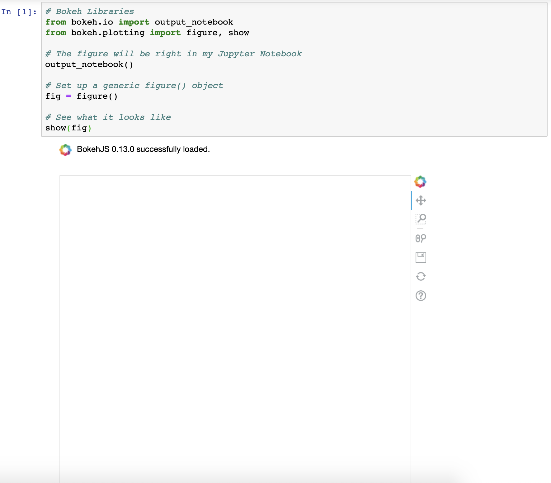
As you can see, the result is the same, just rendered in a different location.
More information about both output_file() and output_notebook() can be found in the Bokeh official docs.
Note: Sometimes, when rendering multiple visualizations sequentially, you’ll see that past renders are not being cleared with each execution. If you experience this, import and run the following between executions:
# Import reset_output (only needed once) frombokeh.plottingimportreset_output# Use reset_output() between subsequent show() calls, as neededreset_output()Before moving on, you may have noticed that the default Bokeh figure comes pre-loaded with a toolbar. This is an important sneak preview into the interactive elements of Bokeh that come right out of the box. You’ll find out more about the toolbar and how to configure it in the Adding Interaction section at the end of this tutorial.
Getting Your Figure Ready for Data
Now that you know how to create and view a generic Bokeh figure either in a browser or Jupyter Notebook, it’s time to learn more about how to configure the figure() object.
The figure() object is not only the foundation of your data visualization but also the object that unlocks all of Bokeh’s available tools for visualizing data. The Bokeh figure is a subclass of the Bokeh Plot object, which provides many of the parameters that make it possible to configure the aesthetic elements of your figure.
To show you just a glimpse into the customization options available, let’s create the ugliest figure ever:
# Bokeh Librariesfrombokeh.ioimportoutput_notebookfrombokeh.plottingimportfigure,show# The figure will be rendered inline in my Jupyter Notebookoutput_notebook()# Example figurefig=figure(background_fill_color='gray',background_fill_alpha=0.5,border_fill_color='blue',border_fill_alpha=0.25,plot_height=300,plot_width=500,h_symmetry=True,x_axis_label='X Label',x_axis_type='datetime',x_axis_location='above',x_range=('2018-01-01','2018-06-30'),y_axis_label='Y Label',y_axis_type='linear',y_axis_location='left',y_range=(0,100),title='Example Figure',title_location='right',toolbar_location='below',tools='save')# See what it looks likeshow(fig)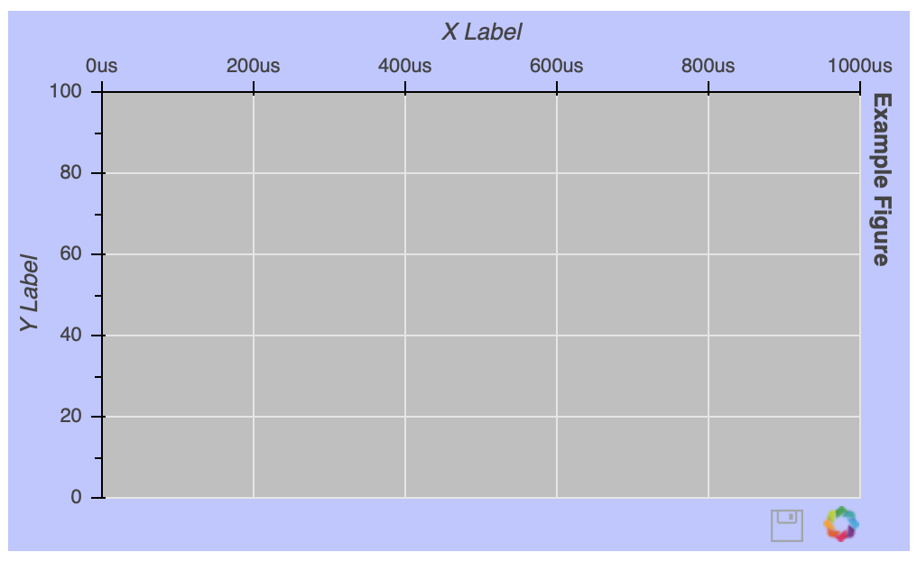
Once the figure() object is instantiated, you can still configure it after the fact. Let’s say you want to get rid of the gridlines:
# Remove the gridlines from the figure() objectfig.grid.grid_line_color=None# See what it looks like show(fig)The gridline properties are accessible via the figure’s grid attribute. In this case, setting grid_line_color to None effectively removes the gridlines altogether. More details about figure attributes can be found below the fold in the Plot class documentation.
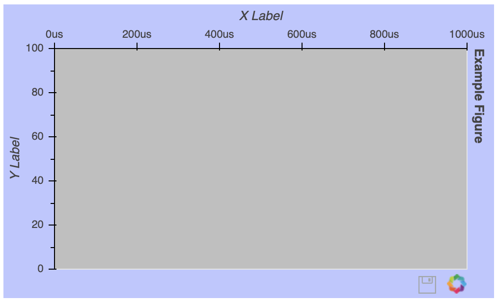
Note: If you’re working in a notebook or IDE with auto-complete functionality, this feature can definitely be your friend! With so many customizable elements, it can be very helpful in discovering the available options:
Otherwise, doing a quick web search, with the keyword bokeh and what you are trying to do, will generally point you in the right direction.
There is tons more I could touch on here, but don’t feel like you’re missing out. I’ll make sure to introduce different figure tweaks as the tutorial progresses. Here are some other helpful links on the topic:
- The Bokeh Plot Class is the superclass of the
figure()object, from which figures inherit a lot of their attributes. - The Figure Class documentation is a good place to find more detail about the arguments of the
figure()object.
Here are a few specific customization options worth checking out:
- Text Properties covers all the attributes related to changing font styles, sizes, colors, and so forth.
- TickFormatters are built-in objects specifically for formatting your axes using Python-like string formatting syntax.
Sometimes, it isn’t clear how your figure needs to be customized until it actually has some data visualized in it, so next you’ll learn how to make that happen.
Drawing Data With Glyphs
An empty figure isn’t all that exciting, so let’s look at glyphs: the building blocks of Bokeh visualizations. A glyph is a vectorized graphical shape or marker that is used to represent your data, like a circle or square. More examples can be found in the Bokeh gallery. After you create your figure, you are given access to a bevy of configurable glyph methods.
Let’s start with a very basic example, drawing some points on an x-y coordinate grid:
# Bokeh Librariesfrombokeh.ioimportoutput_filefrombokeh.plottingimportfigure,show# My x-y coordinate datax=[1,2,1]y=[1,1,2]# Output the visualization directly in the notebookoutput_file('first_glyphs.html',title='First Glyphs')# Create a figure with no toolbar and axis ranges of [0,3]fig=figure(title='My Coordinates',plot_height=300,plot_width=300,x_range=(0,3),y_range=(0,3),toolbar_location=None)# Draw the coordinates as circlesfig.circle(x=x,y=y,color='green',size=10,alpha=0.5)# Show plotshow(fig)
Once your figure is instantiated, you can see how it can be used to draw the x-y coordinate data using customized circle glyphs.
Here are a few categories of glyphs:
Marker includes shapes like circles, diamonds, squares, and triangles and is effective for creating visualizations like scatter and bubble charts.
Line covers things like single, step, and multi-line shapes that can be used to build line charts.
Bar/Rectangle shapes can be used to create traditional or stacked bar (
hbar) and column (vbar) charts as well as waterfall or gantt charts.
Information about the glyphs above, as well as others, can be found in Bokeh’s Reference Guide.
These glyphs can be combined as needed to fit your visualization needs. Let’s say I want to create a visualization that shows how many words I wrote per day to make this tutorial, with an overlaid trend line of the cumulative word count:
importnumpyasnp# Bokeh librariesfrombokeh.ioimportoutput_notebookfrombokeh.plottingimportfigure,show# My word count dataday_num=np.linspace(1,10,10)daily_words=[450,628,488,210,287,791,508,639,397,943]cumulative_words=np.cumsum(daily_words)# Output the visualization directly in the notebookoutput_notebook()# Create a figure with a datetime type x-axisfig=figure(title='My Tutorial Progress',plot_height=400,plot_width=700,x_axis_label='Day Number',y_axis_label='Words Written',x_minor_ticks=2,y_range=(0,6000),toolbar_location=None)# The daily words will be represented as vertical bars (columns)fig.vbar(x=day_num,bottom=0,top=daily_words,color='blue',width=0.75,legend='Daily')# The cumulative sum will be a trend linefig.line(x=day_num,y=cumulative_words,color='gray',line_width=1,legend='Cumulative')# Put the legend in the upper left cornerfig.legend.location='top_left'# Let's check it outshow(fig)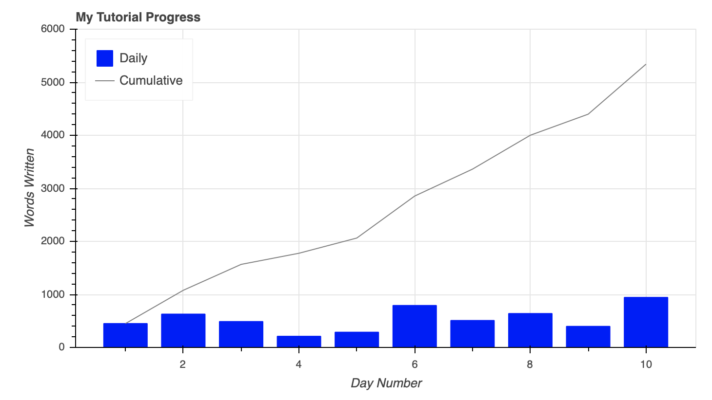
To combine the columns and lines on the figure, they are simply created using the same figure() object.
Additionally, you can see above how seamlessly a legend can be created by setting the legend property for each glyph. The legend was then moved to the upper left corner of the plot by assigning 'top_left' to fig.legend.location.
You can check out much more info about styling legends. Teaser: they will show up again later in the tutorial when we start digging into interactive elements of the visualization.
A Quick Aside About Data
Anytime you are exploring a new visualization library, it’s a good idea to start with some data in a domain you are familiar with. The beauty of Bokeh is that nearly any idea you have should be possible. It’s just a matter of how you want to leverage the available tools to do so.
The remaining examples will use publicly available data from Kaggle, which has information about the National Basketball Association’s (NBA) 2017-18 season, specifically:
- 2017-18_playerBoxScore.csv: game-by-game snapshots of player statistics
- 2017-18_teamBoxScore.csv: game-by-game snapshots of team statistics
- 2017-18_standings.csv: daily team standings and rankings
This data has nothing to do with what I do for work, but I love basketball and enjoy thinking about ways to visualize the ever-growing amount of data associated with it.
If you don’t have data to play with from school or work, think about something you’re interested in and try to find some data related to that. It will go a long way in making both the learning and the creative process faster and more enjoyable!
To follow along with the examples in the tutorial, you can download the datasets from the links above and read them into a Pandas DataFrame using the following commands:
importpandasaspd# Read the csv filesplayer_stats=pd.read_csv('2017-18_playerBoxScore.csv',parse_dates=['gmDate'])team_stats=pd.read_csv('2017-18_teamBoxScore.csv',parse_dates=['gmDate'])standings=pd.read_csv('2017-18_standings.csv',parse_dates=['stDate'])This code snippet reads the data from the three CSV files and automatically interprets the date columns as datetime objects.
It’s now time to get your hands on some real data.
Using the ColumnDataSource Object
The examples above used Python lists and Numpy arrays to represent the data, and Bokeh is well equipped to handle these datatypes. However, when it comes to data in Python, you are most likely going to come across Python dictionaries and Pandas DataFrames, especially if you’re reading in data from a file or external data source.
Bokeh is well equipped to work with these more complex data structures and even has built-in functionality to handle them, namely the ColumnDataSource.
You may be asking yourself, “Why use a ColumnDataSource when Bokeh can interface with other data types directly?”
For one, whether you reference a list, array, dictionary, or DataFrame directly, Bokeh is going to turn it into a ColumnDataSource behind the scenes anyway. More importantly, the ColumnDataSource makes it much easier to implement Bokeh’s interactive affordances.
The ColumnDataSource is foundational in passing the data to the glyphs you are using to visualize. Its primary functionality is to map names to the columns of your data. This makes it easier for you to reference elements of your data when building your visualization. It also makes it easier for Bokeh to do the same when building your visualization.
The ColumnDataSource can interpret three types of data objects:
Python
dict: The keys are names associated with the respective value sequences (lists, arrays, and so forth).Pandas
DataFrame: The columns of theDataFramebecome the reference names for theColumnDataSource.Pandas
groupby: The columns of theColumnDataSourcereference the columns as seen by callinggroupby.describe().
Let’s start by visualizing the race for first place in the NBA’s Western Conference in 2017-18 between the defending champion Golden State Warriors and the challenger Houston Rockets. The daily win-loss records of these two teams is stored in a DataFrame named west_top_2:
>>>
>>> west_top_2=(standings[(standings['teamAbbr']=='HOU')|(standings['teamAbbr']=='GS')]... .loc[:,['stDate','teamAbbr','gameWon']]... .sort_values(['teamAbbr','stDate']))>>> west_top_2.head() stDate teamAbbr gameWon9 2017-10-17 GS 039 2017-10-18 GS 069 2017-10-19 GS 099 2017-10-20 GS 1129 2017-10-21 GS 1
From here, you can load this DataFrame into two ColumnDataSource objects and visualize the race:
# Bokeh librariesfrombokeh.plottingimportfigure,showfrombokeh.ioimportoutput_filefrombokeh.modelsimportColumnDataSource# Output to fileoutput_file('west-top-2-standings-race.html',title='Western Conference Top 2 Teams Wins Race')# Isolate the data for the Rockets and Warriorsrockets_data=west_top_2[west_top_2['teamAbbr']=='HOU']warriors_data=west_top_2[west_top_2['teamAbbr']=='GS']# Create a ColumnDataSource object for each teamrockets_cds=ColumnDataSource(rockets_data)warriors_cds=ColumnDataSource(warriors_data)# Create and configure the figurefig=figure(x_axis_type='datetime',plot_height=300,plot_width=600,title='Western Conference Top 2 Teams Wins Race, 2017-18',x_axis_label='Date',y_axis_label='Wins',toolbar_location=None)# Render the race as step linesfig.step('stDate','gameWon',color='#CE1141',legend='Rockets',source=rockets_cds)fig.step('stDate','gameWon',color='#006BB6',legend='Warriors',source=warriors_cds)# Move the legend to the upper left cornerfig.legend.location='top_left'# Show the plotshow(fig)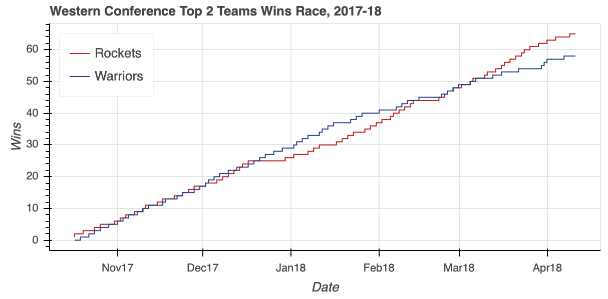
Notice how the respective ColumnDataSource objects are referenced when creating the two lines. You simply pass the original column names as input parameters and specify which ColumnDataSource to use via the source property.
The visualization shows the tight race throughout the season, with the Warriors building a pretty big cushion around the middle of the season. However, a bit of a late-season slide allowed the Rockets to catch up and ultimately surpass the defending champs to finish the season as the Western Conference number-one seed.
Note: In Bokeh, you can specify colors either by name, hex value, or RGB color code.
For the visualization above, a color is being specified for the respective lines representing the two teams. Instead of using CSS color names like 'red' for the Rockets and 'blue' for the Warriors, you might have wanted to add a nice visual touch by using the official team colors in the form of hex color codes. Alternatively, you could have used tuples representing RGB color codes: (206, 17, 65) for the Rockets, (0, 107, 182) for the Warriors.
Bokeh provides a helpful list of CSS color names categorized by their general hue. Also, htmlcolorcodes.com is a great site for finding CSS, hex, and RGB color codes.
ColumnDataSource objects can do more than just serve as an easy way to reference DataFrame columns. The ColumnDataSource object has three built-in filters that can be used to create views on your data using a CDSView object:
GroupFilterselects rows from aColumnDataSourcebased on a categorical reference valueIndexFilterfilters theColumnDataSourcevia a list of integer indicesBooleanFilterallows you to use a list ofbooleanvalues, withTruerows being selected
In the previous example, two ColumnDataSource objects were created, one each from a subset of the west_top_2 DataFrame. The next example will recreate the same output from one ColumnDataSource based on all of west_top_2 using a GroupFilter that creates a view on the data:
# Bokeh librariesfrombokeh.plottingimportfigure,showfrombokeh.ioimportoutput_filefrombokeh.modelsimportColumnDataSource,CDSView,GroupFilter# Output to fileoutput_file('west-top-2-standings-race.html',title='Western Conference Top 2 Teams Wins Race')# Create a ColumnDataSourcewest_cds=ColumnDataSource(west_top_2)# Create views for each teamrockets_view=CDSView(source=west_cds,filters=[GroupFilter(column_name='teamAbbr',group='HOU')])warriors_view=CDSView(source=west_cds,filters=[GroupFilter(column_name='teamAbbr',group='GS')])# Create and configure the figurewest_fig=figure(x_axis_type='datetime',plot_height=300,plot_width=600,title='Western Conference Top 2 Teams Wins Race, 2017-18',x_axis_label='Date',y_axis_label='Wins',toolbar_location=None)# Render the race as step lineswest_fig.step('stDate','gameWon',source=west_cds,view=rockets_view,color='#CE1141',legend='Rockets')west_fig.step('stDate','gameWon',source=west_cds,view=warriors_view,color='#006BB6',legend='Warriors')# Move the legend to the upper left cornerwest_fig.legend.location='top_left'# Show the plotshow(west_fig)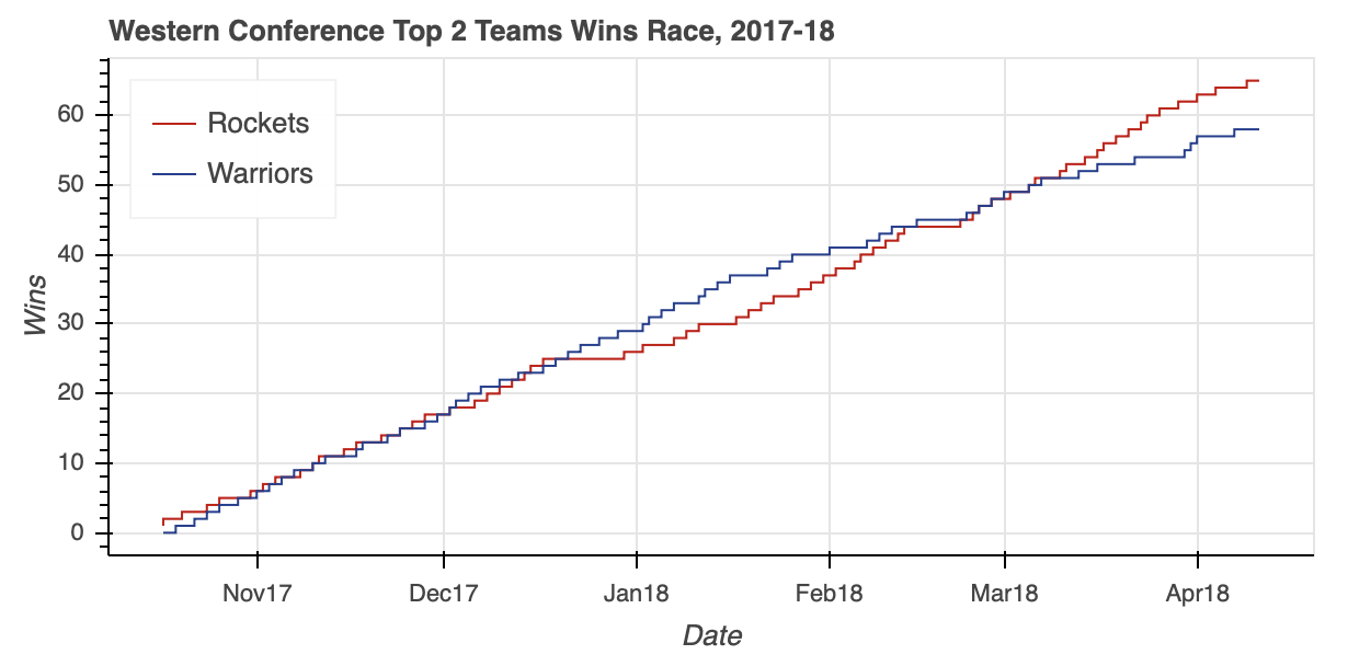
Notice how the GroupFilter is passed to CDSView in a list. This allows you to combine multiple filters together to isolate the data you need from the ColumnDataSource as needed.
For information about integrating data sources, check out the Bokeh user guide’s post on the ColumnDataSource and other source objects available.
The Western Conference ended up being an exciting race, but say you want to see if the Eastern Conference was just as tight. Not only that, but you’d like to view them in a single visualization. This is a perfect segue to the next topic: layouts.
Organizing Multiple Visualizations With Layouts
The Eastern Conference standings came down to two rivals in the Atlantic Division: the Boston Celtics and the Toronto Raptors. Before replicating the steps used to create west_top_2, let’s try to put the ColumnDataSource to the test one more time using what you learned above.
In this example, you’ll see how to feed an entire DataFrame into a ColumnDataSource and create views to isolate the relevant data:
# Bokeh librariesfrombokeh.plottingimportfigure,showfrombokeh.ioimportoutput_filefrombokeh.modelsimportColumnDataSource,CDSView,GroupFilter# Output to fileoutput_file('east-top-2-standings-race.html',title='Eastern Conference Top 2 Teams Wins Race')# Create a ColumnDataSourcestandings_cds=ColumnDataSource(standings)# Create views for each teamceltics_view=CDSView(source=standings_cds,filters=[GroupFilter(column_name='teamAbbr',group='BOS')])raptors_view=CDSView(source=standings_cds,filters=[GroupFilter(column_name='teamAbbr',group='TOR')])# Create and configure the figureeast_fig=figure(x_axis_type='datetime',plot_height=300,plot_width=600,title='Eastern Conference Top 2 Teams Wins Race, 2017-18',x_axis_label='Date',y_axis_label='Wins',toolbar_location=None)# Render the race as step lineseast_fig.step('stDate','gameWon',color='#007A33',legend='Celtics',source=standings_cds,view=celtics_view)east_fig.step('stDate','gameWon',color='#CE1141',legend='Raptors',source=standings_cds,view=raptors_view)# Move the legend to the upper left cornereast_fig.legend.location='top_left'# Show the plotshow(east_fig)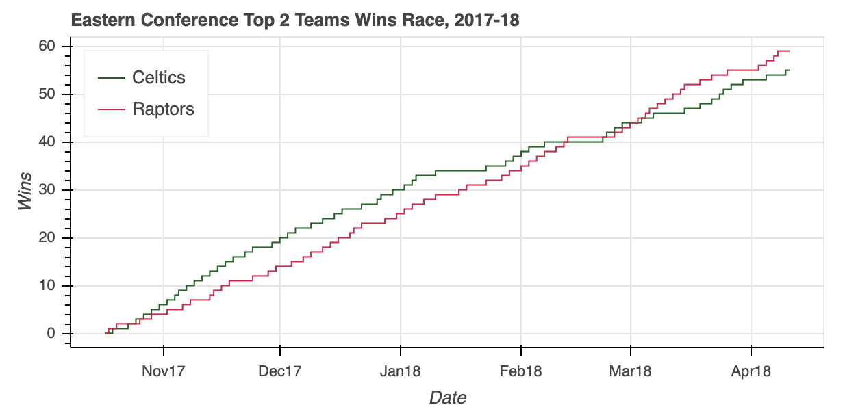
The ColumnDataSource was able to isolate the relevant data within a 5,040-by-39 DataFrame without breaking a sweat, saving a few lines of Pandas code in the process.
Looking at the visualization, you can see that the Eastern Conference race was no slouch. After the Celtics roared out of the gate, the Raptors clawed all the way back to overtake their division rival and finish the regular season with five more wins.
With our two visualizations ready, it’s time to put them together.
Similar to the functionality of Matplotlib’s subplot, Bokeh offers the column, row, and gridplot functions in its bokeh.layouts module. These functions can more generally be classified as layouts.
The usage is very straightforward. If you want to put two visualizations in a vertical configuration, you can do so with the following:
# Bokeh libraryfrombokeh.plottingimportfigure,showfrombokeh.ioimportoutput_filefrombokeh.layoutsimportcolumn# Output to fileoutput_file('east-west-top-2-standings-race.html',title='Conference Top 2 Teams Wins Race')# Plot the two visualizations in a vertical configurationshow(column(west_fig,east_fig))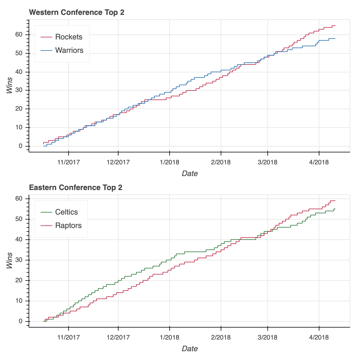
I’ll save you the two lines of code, but rest assured that swapping column for row in the snippet above will similarly configure the two plots in a horizontal configuration.
Note: If you’re trying out the code snippets as you go through the tutorial, I want to take a quick detour to address an error you may see accessing west_fig and east_fig in the following examples. In doing so, you may receive an error like this:
WARNING:bokeh.core.validation.check:W-1004 (BOTH_CHILD_AND_ROOT): Models should not be a document root...This is one of many errors that are part of Bokeh’s validation module, where w-1004 in particular is warning about the re-use of west_fig and east_fig in a new layout.
To avoid this error as you test the examples, preface the code snippet illustrating each layout with the following:
# Bokeh librariesfrombokeh.plottingimportfigure,showfrombokeh.modelsimportColumnDataSource,CDSView,GroupFilter# Create a ColumnDataSourcestandings_cds=ColumnDataSource(standings)# Create the views for each teamceltics_view=CDSView(source=standings_cds,filters=[GroupFilter(column_name='teamAbbr',group='BOS')])raptors_view=CDSView(source=standings_cds,filters=[GroupFilter(column_name='teamAbbr',group='TOR')])rockets_view=CDSView(source=standings_cds,filters=[GroupFilter(column_name='teamAbbr',group='HOU')])warriors_view=CDSView(source=standings_cds,filters=[GroupFilter(column_name='teamAbbr',group='GS')])# Create and configure the figureeast_fig=figure(x_axis_type='datetime',plot_height=300,x_axis_label='Date',y_axis_label='Wins',toolbar_location=None)west_fig=figure(x_axis_type='datetime',plot_height=300,x_axis_label='Date',y_axis_label='Wins',toolbar_location=None)# Configure the figures for each conferenceeast_fig.step('stDate','gameWon',color='#007A33',legend='Celtics',source=standings_cds,view=celtics_view)east_fig.step('stDate','gameWon',color='#CE1141',legend='Raptors',source=standings_cds,view=raptors_view)west_fig.step('stDate','gameWon',color='#CE1141',legend='Rockets',source=standings_cds,view=rockets_view)west_fig.step('stDate','gameWon',color='#006BB6',legend='Warriors',source=standings_cds,view=warriors_view)# Move the legend to the upper left cornereast_fig.legend.location='top_left'west_fig.legend.location='top_left'# Layout code snippet goes here!Doing so will renew the relevant components to render the visualization, ensuring that no warning is needed.
Instead of using column or row, you may want to use a gridplot instead.
One key difference of gridplot is that it will automatically consolidate the toolbar across all of its children figures. The two visualizations above do not have a toolbar, but if they did, then each figure would have its own when using column or row. With that, it also has its own toolbar_location property, seen below set to 'right'.
Syntactically, you’ll also notice below that gridplot differs in that, instead of being passed a tuple as input, it requires a list of lists, where each sub-list represents a row in the grid:
# Bokeh librariesfrombokeh.ioimportoutput_filefrombokeh.layoutsimportgridplot# Output to fileoutput_file('east-west-top-2-gridplot.html',title='Conference Top 2 Teams Wins Race')# Reduce the width of both figureseast_fig.plot_width=west_fig.plot_width=300# Edit the titleseast_fig.title.text='Eastern Conference'west_fig.title.text='Western Conference'# Configure the gridploteast_west_gridplot=gridplot([[west_fig,east_fig]],toolbar_location='right')# Plot the two visualizations in a horizontal configurationshow(east_west_gridplot)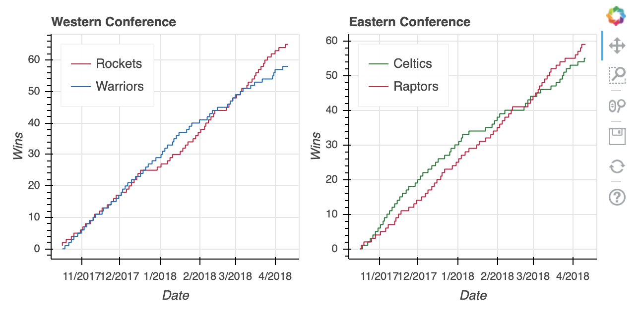
Lastly, gridplot allows the passing of None values, which are interpreted as blank subplots. Therefore, if you wanted to leave a placeholder for two additional plots, then you could do something like this:
# Bokeh librariesfrombokeh.ioimportoutput_filefrombokeh.layoutsimportgridplot# Output to fileoutput_file('east-west-top-2-gridplot.html',title='Conference Top 2 Teams Wins Race')# Reduce the width of both figureseast_fig.plot_width=west_fig.plot_width=300# Edit the titleseast_fig.title.text='Eastern Conference'west_fig.title.text='Western Conference'# Plot the two visualizations with placeholderseast_west_gridplot=gridplot([[west_fig,None],[None,east_fig]],toolbar_location='right')# Plot the two visualizations in a horizontal configurationshow(east_west_gridplot)
If you’d rather toggle between both visualizations at their full size without having to squash them down to fit next to or on top of each other, a good option is a tabbed layout.
A tabbed layout consists of two Bokeh widget functions: Tab() and Panel() from the bokeh.models.widgets sub-module. Like using gridplot(), making a tabbed layout is pretty straightforward:
# Bokeh Libraryfrombokeh.ioimportoutput_filefrombokeh.models.widgetsimportTabs,Panel# Output to fileoutput_file('east-west-top-2-tabbed_layout.html',title='Conference Top 2 Teams Wins Race')# Increase the plot widthseast_fig.plot_width=west_fig.plot_width=800# Create two panels, one for each conferenceeast_panel=Panel(child=east_fig,title='Eastern Conference')west_panel=Panel(child=west_fig,title='Western Conference')# Assign the panels to Tabstabs=Tabs(tabs=[west_panel,east_panel])# Show the tabbed layoutshow(tabs)
The first step is to create a Panel() for each tab. That may sound a little confusing, but think of the Tabs() function as the mechanism that organizes the individual tabs created with Panel().
Each Panel() takes as input a child, which can either be a single figure() or a layout. (Remember that a layout is a general name for a column, row, or gridplot.) Once your panels are assembled, they can be passed as input to Tabs() in a list.
Now that you understand how to access, draw, and organize your data, it’s time to move on to the real magic of Bokeh: interaction! As always, check out Bokeh’s User Guide for more information on layouts.
Adding Interaction
The feature that sets Bokeh apart is its ability to easily implement interactivity in your visualization. Bokeh even goes as far as describing itself as an interactive visualization library:
Bokeh is an interactive visualization library that targets modern web browsers for presentation. (Source)
In this section, we’ll touch on five ways that you can add interactivity:
- Configuring the toolbar
- Selecting data points
- Adding hover actions
- Linking axes and selections
- Highlighting data using the legend
Implementing these interactive elements open up possibilities for exploring your data that static visualizations just can’t do by themselves.
Configuring the Toolbar
As you saw all the way back in Generating Your First Figure, the default Bokeh figure() comes with a toolbar right out of the box. The default toolbar comes with the following tools (from left to right):
- Pan
- Box Zoom
- Wheel Zoom
- Save
- Reset
- A link to Bokeh’s user guide for Configuring Plot Tools
- A link to the Bokeh homepage
The toolbar can be removed by passing toolbar_location=None when instantiating a figure() object, or relocated by passing any of 'above', 'below', 'left', or 'right'.
Additionally, the toolbar can be configured to include any combination of tools you desire. Bokeh offers 18 specific tools across five categories:
- Pan/Drag:
box_select,box_zoom,lasso_select,pan,xpan,ypan,resize_select - Click/Tap:
poly_select,tap - Scroll/Pinch:
wheel_zoom,xwheel_zoom,ywheel_zoom - Actions:
undo,redo,reset,save - Inspectors:
crosshair,hover
To geek out on tools , make sure to visit Specifying Tools. Otherwise, they’ll be illustrated in covering the various interactions covered herein.
Selecting Data Points
Implementing selection behavior is as easy as adding a few specific keywords when declaring your glyphs.
The next example will create a scatter plot that relates a player’s total number of three-point shot attempts to the percentage made (for players with at least 100 three-point shot attempts).
The data can be aggregated from the player_stats DataFrame:
# Find players who took at least 1 three-point shot during the seasonthree_takers=player_stats[player_stats['play3PA']>0]# Clean up the player names, placing them in a single columnthree_takers['name']=[f'{p["playFNm"]}{p["playLNm"]}'for_,pinthree_takers.iterrows()]# Aggregate the total three-point attempts and makes for each playerthree_takers=(three_takers.groupby('name').sum().loc[:,['play3PA','play3PM']].sort_values('play3PA',ascending=False))# Filter out anyone who didn't take at least 100 three-point shotsthree_takers=three_takers[three_takers['play3PA']>=100].reset_index()# Add a column with a calculated three-point percentage (made/attempted)three_takers['pct3PM']=three_takers['play3PM']/three_takers['play3PA']Here’s a sample of the resulting DataFrame:
>>>
>>> three_takers.sample(5) name play3PA play3PM pct3PM229 Corey Brewer 110 31 0.28181878 Marc Gasol 320 109 0.340625126 Raymond Felton 230 81 0.352174127 Kristaps Porziņģis 229 90 0.39301366 Josh Richardson 336 127 0.377976
Let’s say you want to select a groups of players in the distribution, and in doing so mute the color of the glyphs representing the non-selected players:
# Bokeh Librariesfrombokeh.plottingimportfigure,showfrombokeh.ioimportoutput_filefrombokeh.modelsimportColumnDataSource,NumeralTickFormatter# Output to fileoutput_file('three-point-att-vs-pct.html',title='Three-Point Attempts vs. Percentage')# Store the data in a ColumnDataSourcethree_takers_cds=ColumnDataSource(three_takers)# Specify the selection tools to be made availableselect_tools=['box_select','lasso_select','poly_select','tap','reset']# Create the figurefig=figure(plot_height=400,plot_width=600,x_axis_label='Three-Point Shots Attempted',y_axis_label='Percentage Made',title='3PT Shots Attempted vs. Percentage Made (min. 100 3PA), 2017-18',toolbar_location='below',tools=select_tools)# Format the y-axis tick labels as percentagesfig.yaxis[0].formatter=NumeralTickFormatter(format='00.0%')# Add square representing each playerfig.square(x='play3PA',y='pct3PM',source=three_takers_cds,color='royalblue',selection_color='deepskyblue',nonselection_color='lightgray',nonselection_alpha=0.3)# Visualizeshow(fig)First, specify the selection tools you want to make available. In the example above, 'box_select', 'lasso_select', 'poly_select', and 'tap' (plus a reset button) were specified in a list called select_tools. When the figure is instantiated, the toolbar is positioned 'below' the plot, and the list is passed to tools to make the tools selected above available.
Each player is initially represented by a royal blue square glyph, but the following configurations are set for when a player or group of players is selected:
- Turn the selected player(s) to
deepskyblue - Change all non-selected players’ glyphs to a
lightgraycolor with0.3opacity
That’s it! With just a few quick additions, the visualization now looks like this:
For even more information about what you can do upon selection, check out Selected and Unselected Glyphs.
Adding Hover Actions
So the ability to select specific player data points that seem of interest in my scatter plot is implemented, but what if you want to quickly see what individual players a glyph represents? One option is to use Bokeh’s HoverTool() to show a tooltip when the cursor crosses paths with a glyph. All you need to do is append the following to the code snippet above:
# Bokeh Libraryfrombokeh.modelsimportHoverTool# Format the tooltiptooltips=[('Player','@name'),('Three-Pointers Made','@play3PM'),('Three-Pointers Attempted','@play3PA'),('Three-Point Percentage','@pct3PM{00.0%}'),]# Add the HoverTool to the figurefig.add_tools(HoverTool(tooltips=tooltips))# Visualizeshow(fig)The HoverTool() is slightly different than the selection tools you saw above in that it has properties, specifically tooltips.
First, you can configure a formatted tooltip by creating a list of tuples containing a description and reference to the ColumnDataSource. This list was passed as input to the HoverTool() and then simply added to the figure using add_tools(). Here’s what happened:
Notice the addition of the Hover button to the toolbar, which can be toggled on and off.
If you want to even further emphasize the players on hover, Bokeh makes that possible with hover inspections. Here is a slightly modified version of the code snippet that added the tooltip:
# Format the tooltiptooltips=[('Player','@name'),('Three-Pointers Made','@play3PM'),('Three-Pointers Attempted','@play3PA'),('Three-Point Percentage','@pct3PM{00.0%}'),]# Configure a renderer to be used upon hoverhover_glyph=fig.circle(x='play3PA',y='pct3PM',source=three_takers_cds,size=15,alpha=0,hover_fill_color='black',hover_alpha=0.5)# Add the HoverTool to the figurefig.add_tools(HoverTool(tooltips=tooltips,renderers=[hover_glyph]))# Visualizeshow(fig)This is done by creating a completely new glyph, in this case circles instead of squares, and assigning it to hover_glyph. Note that the initial opacity is set to zero so that it is invisible until the cursor is touching it. The properties that appear upon hover are captured by setting hover_alpha to 0.5 along with the hover_fill_color.
Now you will see a small black circle appear over the original square when hovering over the various markers:
To further explore the capabilities of the HoverTool(), see the HoverTool and Hover Inspections guides.
Linking Axes and Selections
Linking is the process of syncing elements of different visualizations within a layout. For instance, maybe you want to link the axes of multiple plots to ensure that if you zoom in on one it is reflected on another. Let’s see how it is done.
For this example, the visualization will be able to pan to different segments of a team’s schedule and examine various game stats. Each stat will be represented by its own plot in a two-by-two gridplot() .
The data can be collected from the team_stats DataFrame, selecting the Philadelphia 76ers as the team of interest:
# Isolate relevant dataphi_gm_stats=(team_stats[(team_stats['teamAbbr']=='PHI')&(team_stats['seasTyp']=='Regular')].loc[:,['gmDate','teamPTS','teamTRB','teamAST','teamTO','opptPTS',]].sort_values('gmDate'))# Add game numberphi_gm_stats['game_num']=range(1,len(phi_gm_stats)+1)# Derive a win_loss columnwin_loss=[]for_,rowinphi_gm_stats.iterrows():# If the 76ers score more points, it's a winifrow['teamPTS']>row['opptPTS']:win_loss.append('W')else:win_loss.append('L')# Add the win_loss data to the DataFramephi_gm_stats['winLoss']=win_lossHere are the results of the 76ers’ first 5 games:
>>>
>>> phi_gm_stats.head() gmDate teamPTS teamTRB teamAST teamTO opptPTS game_num winLoss10 2017-10-18 115 48 25 17 120 1 L39 2017-10-20 92 47 20 17 102 2 L52 2017-10-21 94 41 18 20 128 3 L80 2017-10-23 97 49 25 21 86 4 W113 2017-10-25 104 43 29 16 105 5 L
Start by importing the necessary Bokeh libraries, specifying the output parameters, and reading the data into a ColumnDataSource:
# Bokeh Librariesfrombokeh.plottingimportfigure,showfrombokeh.ioimportoutput_filefrombokeh.modelsimportColumnDataSource,CategoricalColorMapper,Divfrombokeh.layoutsimportgridplot,column# Output to fileoutput_file('phi-gm-linked-stats.html',title='76ers Game Log')# Store the data in a ColumnDataSourcegm_stats_cds=ColumnDataSource(phi_gm_stats)Each game is represented by a column, and will be colored green if the result was a win and red for a loss. To accomplish this, Bokeh’s CategoricalColorMapper can be used to map the data values to specified colors:
# Create a CategoricalColorMapper that assigns a color to wins and losseswin_loss_mapper=CategoricalColorMapper(factors=['W','L'],palette=['green','red'])For this use case, a list specifying the categorical data values to be mapped is passed to factors and a list with the intended colors to palette. For more on the CategoricalColorMapper, see the Colors section of Handling Categorical Data on Bokeh’s User Guide.
There are four stats to visualize in the two-by-two gridplot: points, assists, rebounds, and turnovers. In creating the four figures and configuring their respective charts, there is a lot of redundancy in the properties. So to streamline the code a for loop can be used:
# Create a dict with the stat name and its corresponding column in the datastat_names={'Points':'teamPTS','Assists':'teamAST','Rebounds':'teamTRB','Turnovers':'teamTO',}# The figure for each stat will be held in this dictstat_figs={}# For each stat in the dictforstat_label,stat_colinstat_names.items():# Create a figurefig=figure(y_axis_label=stat_label,plot_height=200,plot_width=400,x_range=(1,10),tools=['xpan','reset','save'])# Configure vbarfig.vbar(x='game_num',top=stat_col,source=gm_stats_cds,width=0.9,color=dict(field='winLoss',transform=win_loss_mapper))# Add the figure to stat_figs dictstat_figs[stat_label]=figAs you can see, the only parameters that needed to be adjusted were the y-axis-label of the figure and the data that will dictate top in the vbar. These values were easily stored in a dict that was iterated through to create the figures for each stat.
You can also see the implementation of the CategoricalColorMapper in the configuration of the vbar glyph. The color property is passed a dict with the field in the ColumnDataSource to be mapped and the name of the CategoricalColorMapper created above.
The initial view will only show the first 10 games of the 76ers’ season, so there needs to be a way to pan horizontally to navigate through the rest of the games in the season. Thus configuring the toolbar to have an xpan tool allows panning throughout the plot without having to worry about accidentally skewing the view along the vertical axis.
Now that the figures are created, gridplot can be setup by referencing the figures from the dict created above:
# Create layoutgrid=gridplot([[stat_figs['Points'],stat_figs['Assists']],[stat_figs['Rebounds'],stat_figs['Turnovers']]])Linking the axes of the four plots is as simple as setting the x_range of each figure equal to one another:
# Link together the x-axesstat_figs['Points'].x_range= \
    stat_figs['Assists'].x_range= \
    stat_figs['Rebounds'].x_range= \
    stat_figs['Turnovers'].x_range
To add a title bar to the visualization, you could have tried to do this on the points figure, but it would have been limited to the space of that figure. Therefore, a nice trick is to use Bokeh’s ability to interpret HTML to insert a Div element that contains the title information. Once that is created, simply combine that with the gridplot() in a column layout:
# Add a title for the entire visualization using Divhtml="""<h3>Philadelphia 76ers Game Log</h3><b><i>2017-18 Regular Season</i><br></b><i>Wins in green, losses in red</i>"""sup_title=Div(text=html)# Visualizeshow(column(sup_title,grid))Putting all the pieces together results in the following:
Similarly you can easily implement linked selections, where a selection on one plot will be reflected on others.
To see how this works, the next visualization will contain two scatter plots: one that shows the 76ers’ two-point versus three-point field goal percentage and the other showing the 76ers’ team points versus opponent points on a game-by-game basis.
The goal is to be able to select data points on the left-side scatter plot and quickly be able to recognize if the corresponding datapoint on the right scatter plot is a win or loss.
The DataFrame for this visualization is very similar to that from the first example:
# Isolate relevant dataphi_gm_stats_2=(team_stats[(team_stats['teamAbbr']=='PHI')&(team_stats['seasTyp']=='Regular')].loc[:,['gmDate','team2P%','team3P%','teamPTS','opptPTS']].sort_values('gmDate'))# Add game numberphi_gm_stats_2['game_num']=range(1,len(phi_gm_stats_2)+1)# Derive a win_loss columnwin_loss=[]for_,rowinphi_gm_stats_2.iterrows():# If the 76ers score more points, it's a winifrow['teamPTS']>row['opptPTS']:win_loss.append('W')else:win_loss.append('L')# Add the win_loss data to the DataFramephi_gm_stats_2['winLoss']=win_lossHere’s what the data looks like:
>>>
>>> phi_gm_stats_2.head() gmDate team2P% team3P% teamPTS opptPTS game_num winLoss10 2017-10-18 0.4746 0.4286 115 120 1 L39 2017-10-20 0.4167 0.3125 92 102 2 L52 2017-10-21 0.4138 0.3333 94 128 3 L80 2017-10-23 0.5098 0.3750 97 86 4 W113 2017-10-25 0.5082 0.3333 104 105 5 L
The code to create the visualization is as follows:
# Bokeh Librariesfrombokeh.plottingimportfigure,showfrombokeh.ioimportoutput_filefrombokeh.modelsimportColumnDataSource,CategoricalColorMapper,NumeralTickFormatterfrombokeh.layoutsimportgridplot# Output inline in the notebookoutput_file('phi-gm-linked-selections.html',title='76ers Percentages vs. Win-Loss')# Store the data in a ColumnDataSourcegm_stats_cds=ColumnDataSource(phi_gm_stats_2)# Create a CategoricalColorMapper that assigns specific colors to wins and losseswin_loss_mapper=CategoricalColorMapper(factors=['W','L'],palette=['Green','Red'])# Specify the toolstoolList=['lasso_select','tap','reset','save']# Create a figure relating the percentagespctFig=figure(title='2PT FG % vs 3PT FG %, 2017-18 Regular Season',plot_height=400,plot_width=400,tools=toolList,x_axis_label='2PT FG%',y_axis_label='3PT FG%')# Draw with circle markerspctFig.circle(x='team2P%',y='team3P%',source=gm_stats_cds,size=12,color='black')# Format the y-axis tick labels as percenagespctFig.xaxis[0].formatter=NumeralTickFormatter(format='00.0%')pctFig.yaxis[0].formatter=NumeralTickFormatter(format='00.0%')# Create a figure relating the totalstotFig=figure(title='Team Points vs Opponent Points, 2017-18 Regular Season',plot_height=400,plot_width=400,tools=toolList,x_axis_label='Team Points',y_axis_label='Opponent Points')# Draw with square markerstotFig.square(x='teamPTS',y='opptPTS',source=gm_stats_cds,size=10,color=dict(field='winLoss',transform=win_loss_mapper))# Create layoutgrid=gridplot([[pctFig,totFig]])# Visualizeshow(grid)This is a great illustration of the power in using a ColumnDataSource. As long as the glyph renderers (in this case, the circle glyphs for the percentages, and square glyphs for the wins and losses) share the same ColumnDataSource, then the selections will be linked by default.
Here’s how it looks in action, where you can see selections made on either figure will be reflected on the other:
By selecting a random sample of data points in the upper right quadrant of the left scatter plot, those corresponding to both high two-point and three-point field goal percentage, the data points on the right scatter plot are highlighted.
Similarly, selecting data points on the right scatter plot that correspond to losses tend to be further to the lower left, lower shooting percentages, on the left scatter plot.
All the details on linking plots can be found at Linking Plots in the Bokeh User Guide.
Highlighting Data Using the Legend
That brings us to the final interactivity example in this tutorial: interactive legends.
In the Drawing Data With Glyphs section, you saw how easy it is to implement a legend when creating your plot. With the legend in place, adding interactivity is merely a matter of assigning a click_policy. Using a single line of code, you can quickly add the ability to either hide or mute data using the legend.
In this example, you’ll see two identical scatter plots comparing the game-by-game points and rebounds of LeBron James and Kevin Durant. The only difference will be that one will use a hide as its click_policy, while the other uses mute.
The first step is to configure the output and set up the data, creating a view for each player from the player_stats DataFrame:
# Bokeh Librariesfrombokeh.plottingimportfigure,showfrombokeh.ioimportoutput_filefrombokeh.modelsimportColumnDataSource,CDSView,GroupFilterfrombokeh.layoutsimportrow# Output inline in the notebookoutput_file('lebron-vs-durant.html',title='LeBron James vs. Kevin Durant')# Store the data in a ColumnDataSourceplayer_gm_stats=ColumnDataSource(player_stats)# Create a view for each playerlebron_filters=[GroupFilter(column_name='playFNm',group='LeBron'),GroupFilter(column_name='playLNm',group='James')]lebron_view=CDSView(source=player_gm_stats,filters=lebron_filters)durant_filters=[GroupFilter(column_name='playFNm',group='Kevin'),GroupFilter(column_name='playLNm',group='Durant')]durant_view=CDSView(source=player_gm_stats,filters=durant_filters)Before creating the figures, the common parameters across the figure, markers, and data can be consolidated into dictionaries and reused. Not only does this save redundancy in the next step, but it provides an easy way to tweak these parameters later if need be:
# Consolidate the common keyword arguments in dictscommon_figure_kwargs={'plot_width':400,'x_axis_label':'Points','toolbar_location':None,}common_circle_kwargs={'x':'playPTS','y':'playTRB','source':player_gm_stats,'size':12,'alpha':0.7,}common_lebron_kwargs={'view':lebron_view,'color':'#002859','legend':'LeBron James'}common_durant_kwargs={'view':durant_view,'color':'#FFC324','legend':'Kevin Durant'}Now that the various properties are set, the two scatter plots can be built in a much more concise fashion:
# Create the two figures and draw the datahide_fig=figure(**common_figure_kwargs,title='Click Legend to HIDE Data',y_axis_label='Rebounds')hide_fig.circle(**common_circle_kwargs,**common_lebron_kwargs)hide_fig.circle(**common_circle_kwargs,**common_durant_kwargs)mute_fig=figure(**common_figure_kwargs,title='Click Legend to MUTE Data')mute_fig.circle(**common_circle_kwargs,**common_lebron_kwargs,muted_alpha=0.1)mute_fig.circle(**common_circle_kwargs,**common_durant_kwargs,muted_alpha=0.1)Note that mute_fig has an extra parameter called muted_alpha. This parameter controls the opacity of the markers when mute is used as the click_policy.
Finally, the click_policy for each figure is set, and they are shown in a horizontal configuration:
# Add interactivity to the legendhide_fig.legend.click_policy='hide'mute_fig.legend.click_policy='mute'# Visualizeshow(row(hide_fig,mute_fig))
Once the legend is in place, all you have to do is assign either hide or mute to the figure’s click_policy property. This will automatically turn your basic legend into an interactive legend.
Also note that, specifically for mute, the additional property of muted_alpha was set in the respective circle glyphs for LeBron James and Kevin Durant. This dictates the visual effect driven by the legend interaction.
For more on all things interaction in Bokeh, Adding Interactions in the Bokeh User Guide is a great place to start.
Summary and Next Steps
Congratulations! You’ve made it to the end of this tutorial.
You should now have a great set of tools to start turning your data into beautiful interactive visualizations using Bokeh.
You learned how to:
- Configure your script to render to either a static HTML file or Jupyter Notebook
- Instantiate and customize the
figure()object - Build your visualization using glyphs
- Access and filter your data with the
ColumnDataSource - Organize multiple plots in grid and tabbed layouts
- Add different forms of interaction, including selections, hover actions, linking, and interactive legends
To explore even more of what Bokeh is capable of, the official Bokeh User Guide is an excellent place to dig into some more advanced topics. I’d also recommend checking out Bokeh’s Gallery for tons of examples and inspiration.
[ Improve Your Python With 🐍 Python Tricks 💌 – Get a short & sweet Python Trick delivered to your inbox every couple of days. >> Click here to learn more and see examples ]
↧