We are living in an age of rapidly changing technology. With over 500 programming languages in use globally, it is a dynamic job market for developers. There are pros and cons of all the languages and their adoption is becoming more and more application-specific.
↧
Codementor: Why You Should Learn Several Programming Languages & Where to Learn Them
↧
Paolo Amoroso: How to Use Kivy on Repl.it
I made the Kivy Python cross-platform GUI framework work in a GFX REPL on Repl.it. Repl.it is a multi-language cloud IDE with good support for Python.
To use Kivy on Repl.it, just create a Pygame REPL, which is among the Kivy dependencies, and install Kivy with the package manager or by adding kivy to requirements.txt. Starting such a REPL in a new session takes a while to download and build the required libraries, at least several minutes. So be patient.
This REPL runs the Kivy Showcase, a demo app that showcases some of Kivy’s features.
The demo works fine except for a few overlapping widgets in the top bar. And it has some latency issues, but the poor performance is mostly a consequence of the experimental state of GFX.
If you adjust the handles along the edges of the REPL panes to close all the panes except the app’s, you can use most of the web page area. Here’s a screenshot of what it looks like. I can’t wait for GFX to support running graphical apps as a website, like it’s now possible with terminal apps.
The work of Repl.it user Saibot84 put me on the right track. He experimented with various ways of running Kivy on Repl.it, for example with Polygott and Python REPLs.
Polygott REPLs get stuck when downloading libraries. So I found that the simplest way of running Kivy is to use a Pygame REPL. Unlike Saibot84’s Pygame REPLs, however, it’s unnecessary to explicitly add the Kivy dependencies to requirements.txt, only kivy.
To use Kivy on Repl.it, just create a Pygame REPL, which is among the Kivy dependencies, and install Kivy with the package manager or by adding kivy to requirements.txt. Starting such a REPL in a new session takes a while to download and build the required libraries, at least several minutes. So be patient.
This REPL runs the Kivy Showcase, a demo app that showcases some of Kivy’s features.
The demo works fine except for a few overlapping widgets in the top bar. And it has some latency issues, but the poor performance is mostly a consequence of the experimental state of GFX.
If you adjust the handles along the edges of the REPL panes to close all the panes except the app’s, you can use most of the web page area. Here’s a screenshot of what it looks like. I can’t wait for GFX to support running graphical apps as a website, like it’s now possible with terminal apps.
 |
| The Showcase Kivy demo running on Repl.it maximized in a window by closing all the REPL panes. |
The work of Repl.it user Saibot84 put me on the right track. He experimented with various ways of running Kivy on Repl.it, for example with Polygott and Python REPLs.
Polygott REPLs get stuck when downloading libraries. So I found that the simplest way of running Kivy is to use a Pygame REPL. Unlike Saibot84’s Pygame REPLs, however, it’s unnecessary to explicitly add the Kivy dependencies to requirements.txt, only kivy.
↧
↧
Stack Abuse: Time Series Prediction using LSTM with PyTorch in Python
Time series data, as the name suggests is a type of data that changes with time. For instance, the temperature in a 24-hour time period, the price of various products in a month, the stock prices of a particular company in a year. Advanced deep learning models such as Long Short Term Memory Networks (LSTM), are capable of capturing patterns in the time series data, and therefore can be used to make predictions regarding the future trend of the data. In this article, you will see how to use LSTM algorithm to make future predictions using time series data.
In one of my earlier articles, I explained how to perform time series analysis using LSTM in the Keras library in order to predict future stock prices. In this article, we will be using the PyTorch library, which is one of the most commonly used Python libraries for deep learning.
Before you proceed, it is assumed that you have intermediate level proficiency with the Python programming language and you have installed the PyTorch library. Also, know-how of basic machine learning concepts and deep learning concepts will help. If you have not installed PyTorch, you can do so with the following pip command:
$ pip install pytorch
Dataset and Problem Definition
The dataset that we will be using comes built-in with the Python Seaborn Library. Let's import the required libraries first and then will import the dataset:
import torch
import torch.nn as nn

import seaborn as sns
import numpy as np
import pandas as pd
import matplotlib.pyplot as plt
%matplotlib inline
Let's print the list of all the datasets that come built-in with the Seaborn library:
sns.get_dataset_names()
Output:
['anscombe',
 'attention',
 'brain_networks',
 'car_crashes',
 'diamonds',
 'dots',
 'exercise',
 'flights',
 'fmri',
 'gammas',
 'iris',
 'mpg',
 'planets',
 'tips',
 'titanic']
The dataset that we will be using is the flights dataset. Let's load the dataset into our application and see how it looks:
flight_data = sns.load_dataset("flights")
flight_data.head()
Output:
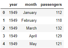
The dataset has three columns: year, month, and passengers. The passengers column contains the total number of traveling passengers in a specified month. Let's plot the shape of our dataset:
flight_data.shape
Output:
(144, 3)
You can see that there are 144 rows and 3 columns in the dataset, which means that the dataset contains 12 year traveling record of the passengers.
The task is to predict the number of passengers who traveled in the last 12 months based on first 132 months. Remember that we have a record of 144 months, which means that the data from the first 132 months will be used to train our LSTM model, whereas the model performance will be evaluated using the values from the last 12 months.
Let's plot the frequency of the passengers traveling per month. The following script increases the default plot size:
fig_size = plt.rcParams["figure.figsize"]
fig_size[0] = 15
fig_size[1] = 5
plt.rcParams["figure.figsize"] = fig_size
And this next script plots the monthly frequency of the number of passengers:
plt.title('Month vs Passenger')
plt.ylabel('Total Passengers')
plt.xlabel('Months')
plt.grid(True)
plt.autoscale(axis='x',tight=True)
plt.plot(flight_data['passengers'])
Output:
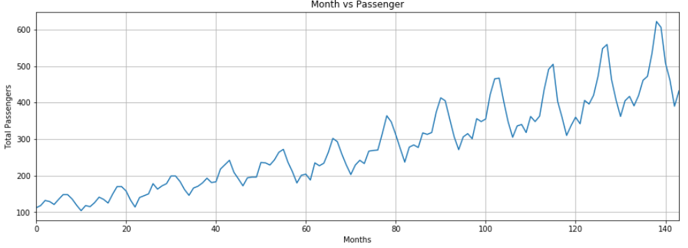
The output shows that over the years the average number of passengers traveling by air increased. The number of passengers traveling within a year fluctuates, which makes sense because during summer or winter vacations, the number of traveling passengers increases compared to the other parts of the year.
Data Preprocessing
The types of the columns in our dataset is object, as shown by the following code:
flight_data.columns
Output:
Index(['year', 'month', 'passengers'], dtype='object')
The first preprocessing step is to change the type of the passengers column to float.
all_data = flight_data['passengers'].values.astype(float)
Now if you print the all_data numpy array, you should see the following floating type values:
print(all_data)
Output:
[112. 118. 132. 129. 121. 135. 148. 148. 136. 119. 104. 118. 115. 126.
 141. 135. 125. 149. 170. 170. 158. 133. 114. 140. 145. 150. 178. 163.
 172. 178. 199. 199. 184. 162. 146. 166. 171. 180. 193. 181. 183. 218.
 230. 242. 209. 191. 172. 194. 196. 196. 236. 235. 229. 243. 264. 272.
 237. 211. 180. 201. 204. 188. 235. 227. 234. 264. 302. 293. 259. 229.
 203. 229. 242. 233. 267. 269. 270. 315. 364. 347. 312. 274. 237. 278.
 284. 277. 317. 313. 318. 374. 413. 405. 355. 306. 271. 306. 315. 301.
 356. 348. 355. 422. 465. 467. 404. 347. 305. 336. 340. 318. 362. 348.
 363. 435. 491. 505. 404. 359. 310. 337. 360. 342. 406. 396. 420. 472.
 548. 559. 463. 407. 362. 405. 417. 391. 419. 461. 472. 535. 622. 606.
 508. 461. 390. 432.]
Next, we will divide our data set into training and test sets. The LSTM algorithm will be trained on the training set. The model will then be used to make predictions on the test set. The predictions will be compared with the actual values in the test set to evaluate the performance of the trained model.
The first 132 records will be used to train the model and the last 12 records will be used as a test set. The following script divides the data into training and test sets.
test_data_size = 12

train_data = all_data[:-test_data_size]
test_data = all_data[-test_data_size:]
Let's now print the length of the test and train sets:
print(len(train_data))
print(len(test_data))
Output:
132
12
If you now print the test data, you will see it contains last 12 records from the all_data numpy array:
print(test_data)
Output:
[417. 391. 419. 461. 472. 535. 622. 606. 508. 461. 390. 432.]
Our dataset is not normalized at the moment. The total number of passengers in the initial years is far less compared to the total number of passengers in the later years. It is very important to normalize the data for time series predictions. We will perform min/max scaling on the dataset which normalizes the data within a certain range of minimum and maximum values. We will be using the MinMaxScaler class from the sklearn.preprocessing module to scale our data. For further details of the min/max scaler implementation, visit this link.
The following code normalizes our data using the min/max scaler with minimum and maximum values of -1 and 1, respectively.
from sklearn.preprocessing import MinMaxScaler

scaler = MinMaxScaler(feature_range=(-1, 1))
train_data_normalized = scaler.fit_transform(train_data .reshape(-1, 1))
Let's now print the first 5 and last 5 records of our normalized train data.
print(train_data_normalized[:5])
print(train_data_normalized[-5:])
Output:
[[-0.96483516]
 [-0.93846154]
 [-0.87692308]
 [-0.89010989]
 [-0.92527473]]
[[1.        ]
 [0.57802198]
 [0.33186813]
 [0.13406593]
 [0.32307692]]
You can see that the dataset values are now between -1 and 1.
It is important to mention here that data normalization is only applied on the training data and not on the test data. If normalization is applied on the test data, there is a chance that some information will be leaked from training set into the test set.
The next step is to convert our dataset into tensors since PyTorch models are trained using tensors. To convert the dataset into tensors, we can simply pass our dataset to the constructor of the FloatTensor object, as shown below:
train_data_normalized = torch.FloatTensor(train_data_normalized).view(-1)
The final preprocessing step is to convert our training data into sequences and corresponding labels.
You can use any sequence length and it depends upon the domain knowledge. However, in our dataset it is convenient to use a sequence length of 12 since we have monthly data and there are 12 months in a year. If we had daily data, a better sequence length would have been 365, i.e. the number of days in a year. Therefore, we will set the input sequence length for training to 12.
train_window = 12
Next, we will define a function named create_inout_sequences. The function will accept the raw input data and will return a list of tuples. In each tuple, the first element will contain list of 12 items corresponding to the number of passengers traveling in 12 months, the second tuple element will contain one item i.e. the number of passengers in the 12+1st month.
def create_inout_sequences(input_data, tw):
    inout_seq = []
    L = len(input_data)
    for i in range(L-tw):
        train_seq = input_data[i:i+tw]
        train_label = input_data[i+tw:i+tw+1]
        inout_seq.append((train_seq ,train_label))
    return inout_seq
Execute the following script to create sequences and corresponding labels for training:
train_inout_seq = create_inout_sequences(train_data_normalized, train_window)
If you print the length of the train_inout_seq list, you will see that it contains 120 items. This is because though the training set contains 132 elements, the sequence length is 12, which means that the first sequence consists of the first 12 items and the 13th item is the label for the first sequence. Similarly, the second sequence starts from the second item and ends at the 13th item, whereas the 14th item is the label for the second sequence and so on.
Let's now print the first 5 items of the train_inout_seq list:
train_inout_seq[:5]
Output:
[(tensor([-0.9648, -0.9385, -0.8769, -0.8901, -0.9253, -0.8637, -0.8066, -0.8066,
          -0.8593, -0.9341, -1.0000, -0.9385]), tensor([-0.9516])),
 (tensor([-0.9385, -0.8769, -0.8901, -0.9253, -0.8637, -0.8066, -0.8066, -0.8593,
          -0.9341, -1.0000, -0.9385, -0.9516]),
  tensor([-0.9033])),
 (tensor([-0.8769, -0.8901, -0.9253, -0.8637, -0.8066, -0.8066, -0.8593, -0.9341,
          -1.0000, -0.9385, -0.9516, -0.9033]), tensor([-0.8374])),
 (tensor([-0.8901, -0.9253, -0.8637, -0.8066, -0.8066, -0.8593, -0.9341, -1.0000,
          -0.9385, -0.9516, -0.9033, -0.8374]), tensor([-0.8637])),
 (tensor([-0.9253, -0.8637, -0.8066, -0.8066, -0.8593, -0.9341, -1.0000, -0.9385,
          -0.9516, -0.9033, -0.8374, -0.8637]), tensor([-0.9077]))]
You can see that each item is a tuple where the first element consists of the 12 items of a sequence, and the second tuple element contains the corresponding label.
Creating LSTM Model
We have preprocessed the data, now is the time to train our model. We will define a class LSTM, which inherits from nn.Module class of the PyTorch library. Check out my last article to see how to create a classification model with PyTorch. That article will help you understand what is happening in the following code.
class LSTM(nn.Module):
    def __init__(self, input_size=1, hidden_layer_size=100, output_size=1):
        super().__init__()
        self.hidden_layer_size = hidden_layer_size

        self.lstm = nn.LSTM(input_size, hidden_layer_size)

        self.linear = nn.Linear(hidden_layer_size, output_size)

        self.hidden_cell = (torch.zeros(1,1,self.hidden_layer_size),
                            torch.zeros(1,1,self.hidden_layer_size))

    def forward(self, input_seq):
        lstm_out, self.hidden_cell = self.lstm(input_seq.view(len(input_seq) ,1, -1), self.hidden_cell)
        predictions = self.linear(lstm_out.view(len(input_seq), -1))
        return predictions[-1]
Let me summarize what is happening in the above code. The constructor of the LSTM class accepts three parameters:
input_size: Corresponds to the number of features in the input. Though our sequence length is 12, for each month we have only 1 value i.e. total number of passengers, therefore the input size will be 1.hidden_layer_size: Specifies the number of hidden layers along with the number of neurons in each layer. We will have one layer of 100 neurons.output_size: The number of items in the output, since we want to predict the number of passengers for 1 month in the future, the output size will be 1.
Next, in the constructor we create variables hidden_layer_size, lstm, linear, and hidden_cell. LSTM algorithm accepts three inputs: previous hidden state, previous cell state and current input. The hidden_cell variable contains the previous hidden and cell state. The lstm and linear layer variables are used to create the LSTM and linear layers.
Inside the forward method, the input_seq is passed as a parameter, which is first passed through the lstm layer. The output of the lstm layer is the hidden and cell states at current time step, along with the output. The output from the lstm layer is passed to the linear layer. The predicted number of passengers is stored in the last item of the predictions list, which is returned to the calling function.
The next step is to create an object of the LSTM() class, define a loss function and the optimizer. Since, we are solving a classification problem, we will use the cross entropy loss. For the optimizer function, we will use the adam optimizer.
model = LSTM()
loss_function = nn.MSELoss()
optimizer = torch.optim.Adam(model.parameters(), lr=0.001)
Let's print our model:
print(model)
Output:
LSTM(
  (lstm): LSTM(1, 100)
  (linear): Linear(in_features=100, out_features=1, bias=True)
)
Training the Model
We will train our model for 150 epochs. You can try with more epochs if you want. The loss will be printed after every 25 epochs.
epochs = 150

for i in range(epochs):
    for seq, labels in train_inout_seq:
        optimizer.zero_grad()
        model.hidden_cell = (torch.zeros(1, 1, model.hidden_layer_size),
                        torch.zeros(1, 1, model.hidden_layer_size))

        y_pred = model(seq)

        single_loss = loss_function(y_pred, labels)
        single_loss.backward()
        optimizer.step()

    if i%25 == 1:
        print(f'epoch: {i:3} loss: {single_loss.item():10.8f}')

print(f'epoch: {i:3} loss: {single_loss.item():10.10f}')
Output:
epoch:   1 loss: 0.00517058
epoch:  26 loss: 0.00390285
epoch:  51 loss: 0.00473305
epoch:  76 loss: 0.00187001
epoch: 101 loss: 0.00000075
epoch: 126 loss: 0.00608046
epoch: 149 loss: 0.0004329932
You may get different values since by default weights are initialized randomly in a PyTorch neural network.
Making Predictions
Now that our model is trained, we can start to make predictions. Since our test set contains the passenger data for the last 12 months and our model is trained to make predictions using a sequence length of 12. We will first filter the last 12 values from the training set:
fut_pred = 12

test_inputs = train_data_normalized[-train_window:].tolist()
print(test_inputs)
Output:
[0.12527473270893097, 0.04615384712815285, 0.3274725377559662, 0.2835164964199066, 0.3890109956264496, 0.6175824403762817, 0.9516483545303345, 1.0, 0.5780220031738281, 0.33186814188957214, 0.13406594097614288, 0.32307693362236023]
You can compare the above values with the last 12 values of the train_data_normalized data list.
Initially the test_inputs item will contain 12 items. Inside a for loop these 12 items will be used to make predictions about the first item from the test set i.e. the item number 133. The predict value will then be appended to the test_inputs list. During the second iteration, again the last 12 items will be used as input and a new prediction will be made which will then be appended to the test_inputs list again. The for loop will execute for 12 times since there are 12 elements in the test set. At the end of the loop the test_inputs list will contain 24 items. The last 12 items will be the predicted values for the test set.
The following script is used to make predictions:
model.eval()

for i in range(fut_pred):
    seq = torch.FloatTensor(test_inputs[-train_window:])
    with torch.no_grad():
        model.hidden = (torch.zeros(1, 1, model.hidden_layer_size),
                        torch.zeros(1, 1, model.hidden_layer_size))
        test_inputs.append(model(seq).item())
If you print the length of the test_inputs list, you will see it contains 24 items. The last 12 predicted items can be printed as follows:
test_inputs[fut_pred:]
Output:
[0.4574652910232544,
 0.9810629487037659,
 1.279405951499939,
 1.0621851682662964,
 1.5830546617507935,
 1.8899496793746948,
 1.323508620262146,
 1.8764172792434692,
 2.1249167919158936,
 1.7745600938796997,
 1.7952896356582642,
 1.977765679359436]
It is pertinent to mention again that you may get different values depending upon the weights used for training the LSTM.
Since we normalized the dataset for training, the predicted values are also normalized. We need to convert the normalized predicted values into actual predicted values. We can do so by passing the normalized values to the inverse_transform method of the min/max scaler object that we used to normalize our dataset.
actual_predictions = scaler.inverse_transform(np.array(test_inputs[train_window:] ).reshape(-1, 1))
print(actual_predictions)
Output:
[[435.57335371]
 [554.69182083]
 [622.56485397]
 [573.14712578]
 [691.64493555]
 [761.46355206]
 [632.59821111]
 [758.38493103]
 [814.91857016]
 [735.21242136]
 [739.92839211]
 [781.44169205]]
Let's now plot the predicted values against the actual values. Look at the following code:
x = np.arange(132, 144, 1)
print(x)
Output:
[132 133 134 135 136 137 138 139 140 141 142 143]
In the script above we create a list that contains numeric values for the last 12 months. The first month has an index value of 0, therefore the last month will be at index 143.
In the following script, we will plot the total number of passengers for 144 months, along with the predicted number of passengers for the last 12 months.
plt.title('Month vs Passenger')
plt.ylabel('Total Passengers')
plt.grid(True)
plt.autoscale(axis='x', tight=True)
plt.plot(flight_data['passengers'])
plt.plot(x,actual_predictions)
plt.show()
Output:
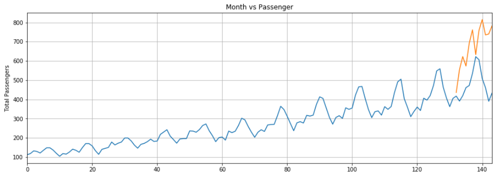
The predictions made by our LSTM are depicted by the orange line. You can see that our algorithm is not too accurate but still it has been able to capture upward trend for total number of passengers traveling in the last 12 months along with occasional fluctuations. You can try with a greater number of epochs and with a higher number of neurons in the LSTM layer to see if you can get better performance.
To have a better view of the output, we can plot the actual and predicted number of passengers for the last 12 months as follows:
plt.title('Month vs Passenger')
plt.ylabel('Total Passengers')
plt.grid(True)
plt.autoscale(axis='x', tight=True)

plt.plot(flight_data['passengers'][-train_window:])
plt.plot(x,actual_predictions)
plt.show()
Output:
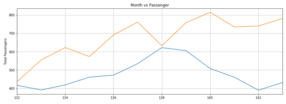
Again, the predictions are not very accurate but the algorithm was able to capture the trend that the number of passengers in the future months should be higher than the previous months with occasional fluctuations.
Conclusion
LSTM is one of the most widely used algorithm to solve sequence problems. In this article we saw how to make future predictions using time series data with LSTM. You also saw how to implement LSTM with PyTorch library and then how to plot predicted results against actual values to see how well the trained algorithm is performing.
↧
Samuel Sutch: Coding for Kids: Python: Learn to Code with 50 Awesome Games and Activities
Price: $13.53
(as of Oct 25,2019 21:52:25 UTC – Details)

“Python is a really powerful programming language with very simple and human-like syntax. Thanks to these advantages and the interactive exercises and games in Coding for Kids: Python, everyone—regardless of age—will be able to understand the power of the language and start using it immediately. I really can’t wait to use some of these examples in our school!”—Marcin Zajkowski, Co-owner of WOW School
↧
Samuel Sutch: Programming the Raspberry Pi, Second Edition: Getting Started with Python
Price: $11.99
(as of Oct 25,2019 23:58:15 UTC – Details)
Dr. Simon Monk has a bachelor’s degree in cybernetics and computer science and a Ph.D. in software engineering. He is now a full-time writer and has authored numerous books, including Programming Arduino, 30 Arduino Projects for the Evil Genius, Hacking Electronics, and Fritzing for Inventors. Dr. Monk also runs the website monk.makes.com, which features his own products.
↧
↧
Samuel Sutch: Learn Robotics Programming: Build and control autonomous robots using Raspberry Pi 3 and Python
Price: $39.99
(as of Oct 26,2019 06:03:34 UTC – Details)
Danny Staple builds robots and gadgets as a hobbyist, makes videos about his work with robots, and attends community events such as PiWars and Arduino Day. He has been a professional Python programmer, later moving into DevOps, since 2009, and a software engineer since 2000. He has worked with embedded systems, including embedded Linux systems, throughout the majority of his career. He has been a mentor at a local CoderDojo, where he taught how to code with Python. He has run Lego Robotics clubs with Mindstorms. He has also developed Bounce!, a visual programming language targeted at teaching code using the NodeMCU IoT platform.
The robots he has built with his children include TankBot, SkittleBot (now the Pi Wars robot), ArmBot, and SpiderBot.
↧
Catalin George Festila: Python 3.7.4 : About with the PyOpenCL python module.
PyOpenCL lets you access GPUs and other massively parallel compute devices from Python.
It is important to note that OpenCL is not restricted to GPUs.
In fact, no special hardware is required to use OpenCL for computation–your existing CPU is enough.
The documentation of this project can be found at this website.
Let's install the python module for python 3 version:
[mythcat@desk ~]$ pip3 install
↧
Samuel Sutch: Murach’s Python Programming
Price: $44.38
(as of Oct 26,2019 22:15:33 UTC – Details)
Section 1 Essential concepts and skills
Chapter 1 An introduction to Python programming
Chapter 2 How to write your first programs
Chapter 3 How to code control statements
Chapter 4 How to define and use functions and modules
Chapter 5 How to test and debug a program
Chapter 6 How to work with lists and tuples
Chapter 7 How to work with file I/O
Chapter 8 How to handle exceptions
Section 2 Other concepts and skills
Chapter 9 How to work with numbers
Chapter 10 How to work with strings
Chapter 11 How to work with dates and times
Chapter 12 How to work with dictionaries
Chapter 13 How to work with recursion and algorithms
Section 3 Object-oriented programming
Chapter 14 How to define and use your own classes
Chapter 15 How to work with inheritance
Chapter 16 How to design an object-oriented program
Section 4 Database and GUI programming
Chapter 17 How to work with a database
Chapter 18 How to build a GUI program
↧
Brett Cannon: What it's like to be on the Python steering council
Someone emailed the steering council recently to ask what it was like to be on it, presumably because nominations will be opening next month. Instead of sending a private response I figured I would write a blog post instead so others could know what it's like after 10 months on the inaugural council.
What we do
Basically what we do is either reactive or proactive. I can't actually provide an estimate of where the balance lands because it very much depends on what comes up reactively.
Reactive
The reactive bit revolves around the council being the "higher power" for the Python development team to appeal to. That means we do things like discuss PEPs as we will ultimately be the ones who are asked to either name a BDFL-Delegate or rule on the PEP as a council (which is typically what happens if any one of us on the council is named the BDFL-Delegate; we are at that point acting as point person for the council on that PEP). We also get asked to deal with anything where a stalemate has been reached in a discussion and the status quo is not really an option. Lastly, there are some sensitive issues that do come up team-wise and we have to deal with those to varying degrees.
Proactive
When we are not reacting to something that is brought to our attention we try to do what we can to help keep the Python project running. In terms of PEPs that means we try to nudge any along that seem to have gone quiet for a period of time as well as shut down any early on if we think they have no chance of acceptance.
We also start projects on our own which we are in a unique position to help with. A good example of this is making sure the new PSF Code of Conduct would work for the Python development team and then making sure it applied to the development of Python. We've also thought of, worked out, and got the PSF to hire a project manager to help manage the sunsetting of Python 2 so that it wasn't just an abrupt shutdown come 2020. (We're also working on some other stuff but this post isn't about what we are doing so I'm going to cut the list short.)
How much time it takes
The time commitment to being on the council could be broken down to simply being on the council and then being an active Python development team member. For the former there's the weekly, hour-long meeting over video chat we hold as well as any preparation each of us need to do for that meeting. There's also any work to be done for the projects we have going on. All of that is probably about 3 hours each week.
But then there's being a participating member of the Python development team on top of it all. That means keeping up with python-committers/discuss.python.org, python-dev, and python-ideas to some extent. I would say that since the steering council is meant to be the backstop to the project it means you should have a wide understanding of what is going on overall in the project and with the overall community. That's its own time commitment and I don't really have a good handle on how much time that takes for me personally, but a wild guess is roughly 4 hours/week if I don't get pulled into some coding task or thread that leads to deep engagement.
So in total I would guess I spend about 7 - 8 hours/week on steering council + Python dev stuff, another 4 -8 hours for everything else Python-related that I do, e.g. my participation in the packaging side of things. (Massive thanks to Microsoft for giving me work time to do this stuff.)
↧
↧
Weekly Python StackOverflow Report: (cc) stackoverflow python report
These are the ten most rated questions at Stack Overflow last week.
Between brackets: [question score / answers count]
Build date: 2019-10-27 06:20:02 GMT
- Get overridden functions of subclass - [15/4]
- numpy 1D array: mask elements that repeat more than n times - [14/8]
- Tuple slicing not returning a new object as opposed to list slicing - [11/4]
- Are there some a, b such that max(a, b) != max(b, a)? - [9/2]
- I happen to stumble upon this code :" With for w in words:, the example would attempt to create an infinite list - [6/2]
- Merge two data frames with the closest number into a single row using pandas? - [6/1]
- How to fade the screen out and back in using PyGame? - [6/1]
- How to create JPEG compressed DICOM dataset using pydicom? - [6/0]
- Iterate through string and print distance between characters - [5/5]
- split rows in pandas dataframe - [5/4]
↧
Samuel Sutch: Python Geospatial Analysis Cookbook
Price: $49.99
(as of Oct 27,2019 14:35:09 UTC – Details)
Michael Diener
↧
Python Diary: Python and Docker development
As I will be starting a new full-time job soon which will be using Docker as their primary deployment technology, I thought this would be the best time to jump back into Docker to see what has changed over the years since I tried it last. It has definitely evolved into a much more useful product, and if used correctly in practice, it can be extremely powerful. Here are some bullet point use-cases for Docker I can think of:
- Server software isolation in a powerful cgroup-enabled chroot jail
- Self-contained development environments which can be easily shared
- Support legacy Linux server software in a safely contained environment
- Running programs using a completely different Linux distribution
- Scaling out a large microservice stack using either Swarm or Kubernetes
Now, Docker isn't with it's security flaws as I recently found out. Basically, if a hacker gains access to an account which is part of the docker group on Linux, they can easily gain full root access to that system. Some may argue however, that once a hacker does get in, it is normally best to completely wipe that machine and reinstall from scratch, as there is no telling what the hacker may have done, or exploited. However, it is still best to have proper barriers in place to prevent an unauthorized person from gaining root in the first place. This way, you can still recover whatever data is on that machine with at least some certainty that it has not been tampered with. You will of course want to scrub said data and perhaps compare it to a recent backup to confirm it can be imported into the newly created machine. Basically, any user in the docker group on Linux has full access to the docker daemon to manage the images and containers. With this ability, you easily use a bind volume to map the entire root file system into the docker container, which will actually then give you full read/write access to the entire system. A hacker can then proceed to change the root password, modify various system files, and generally cause damage which could have otherwise been avoided if docker wasn't exposed. When I normally configure a Linux server, I do not install sudo, or any packages which otherwise could be abused to gain root. However, I am soon planning on using Docker on my current cloud servers as a partial experiment, and partially because I do not have enough time to upgrade my software from an aging Debian server. However, I will not be placing any user in the docker group, and instead using the stellar SaltStack, and their docker states to configure the containers on the cloud server. This provides a nice isolation between user and system processes.
However, you aren't here to read about the use-cases of Docker, or hear me ramble on about it's potential security flaws if not configured correctly. You are here to read about how you can use Docker with a local Python development environment. If you are in a position where you are putting together docker images for an organization, here is a word of advise, I would not recommend using the various software images on the Docker Hub. You may be asking, why's that? There are plenty of pre-created images you can easily pull in and use. The problem with this, is efficiency. If you do not have a hugely large stack, or are just playing around with various software trying to learn it, then pulling images from Docker Hub is perfectly fine. However, for production servers, you always want to aim for the most efficient method to allow your application stack to easily scale without worry. If you pull images from Docker Hub, you will have a large number of incompatible base images, leading to a large amount of downloads, and a large amounts of customizations on your part. As time goes on, you may find it getting very difficult to manage all these various images. My suggestion is to use a base operating system image with lots to offer. I personally use Debian, so I spin my images from a base Debian image, which I do pull from Docker Hub. From this, I make a simple customization to point the Debian mirror to my local mirror to drastically speed up docker image building. My absolute base image is a Debian image with a simple mirror customization in it. I then build on top of this with the various base software packages I will be needing, and create several custom images from that. The reason is this much more efficient than pulling random images from Docker Hub is simple, local disk and memory caches. Also, if you opt for ZFS, this can be a huge savings in both space and overall performance of your images, as all your software is sharing the same sectors on the underlying disk media. This along with disk and memory caching, allows the various shared libraries from your ultimate base image to be easily shared and managed by the host kernel, leading to lower memory and disk usage. As your application stack grows, memory and disk will start to mean more, and have an effect on the application's overall performance.
And there I go rambling again... Let's get started with a custom Dockerfile I created to enable easier development with Django. Both this Dockerfile and the entrypoint script can be updated for your specific use-cases, feel free to use them as you please.
FROM python:2.7.9


RUN pip install Django==1.11.17


ADD entrypoint.py /


VOLUME /app


EXPOSE 8000


ENTRYPOINT ["/entrypoint.py"]
Yes, I know, Python 2.7.x is losing support as of January, 2020. As stated above, please customize for your own use-cases. The above Python image may not exist in Docker Hub, so either roll your own base image, or update that line to point to an acceptable image. Next, let's take a look at the entrypoint script:
#!/usr/bin/pythonimportsys,os,djangoprint"Kevin's Django Development Docker Image\n\n"print"Django Version: %s"%django.get_version()print"PID: %s"%os.getpid()app_dir=os.listdir('/app')iflen(app_dir)==0:print" *** No Django Project currently exists! ***"proj_dir=Noneelse:fordinapp_dir:ifd=='requirements.txt':os.system('pip install -r /app/requirements.txt')else:try:os.stat('/app/%s/manage.py'%d)print"Found Project: %s"%dproj_dir='/app/%s'%dexcept:passifproj_dir:os.chdir(proj_dir)else:os.chdir('/app')params=len(sys.argv)ifparams==1:ifproj_dir:args=['/usr/bin/python','%s/manage.py'%proj_dir,'runserver','0.0.0.0:8000']else:sys.exit(2)else:ifsys.argv[1]=='bash':os.execl('/bin/bash','bash')elifsys.argv[1]=='startproject':ifproj_dir:print" *** The project directory '%s' already exists! ***"%proj_dirsys.exit(2)ifparams!=3:print" *** Missing parameter to startproject! ***"sys.exit(2)args=['django-admin','/usr/local/bin/django-admin.py','startproject',sys.argv[2]]else:args=['manage.py','%s/manage.py'%proj_dir]+sys.argv[1:]os.execv('/usr/bin/python',args)If you are using Python 3, update the print statements and anything else which is needed. This entrypoint script is very tailored towards Django development as you may see. It does quite a few checks within the /app directory. It will check for a requirements.txt file, and install the packages into the container, and attempt to auto-detect the Django project directory by searching for manage.py. Depending on if a Django project is found, it will allow the use of startproject, or allow you to call sub-commands of the manage.py command effortlessly. The idea is that you use a bind volume map to your host file system where your Django project lives. This allows you to easily develop using your favorite IDE on your host machine, while keeping a very persistent development environment within the container itself. I even created a nice shell script to allow the starting of this development environment with zero efforts.
#!/bin/shPROJ_DIR=$1shift

docker run -it -v $PROJ_DIR:/app -p 8000:8000 --rm django:dev "$@"
This could be updated to allow the port to be changed and such as well. You can run this within the project directory and pass `pwd` for example to have it use the current directory. This ensures a pristine start everytime, so you know that the packages in the environment always match.
In the next article I will be publish shortly, I will provide another Dockerfile and an endpoint.py file which will allow you to run any Python web framework from the powerful uWSGI container software within a Docker container.
↧
Python Diary: Deploying with Docker and uWSGI
While I am not going to say that I am expert with Docker by any means. This is just an analysis and example on how I plan on deploying uWSGI containers within Docker containers. I highly recommend reading my previous article from today for some additional context on my thoughts behind docker. With that said, let's get started.
While Gunicorn seems to be much more popular than uWSGI when it comes to deploying Python web applications, I still prefer the extremely power uWSGI, as it has full integration with the nginx web server, which is my preferred web server of choice. uWSGI has a great plugin system, and has a really powerful load balancer and application router built right in. Let's get down to business here and I'll show you my custom Dockerfile for deploying uWSGI applications:
FROM python:2.7.9


RUN apt-get update && apt-get -y install uwsgi-core uwsgi-plugin-python


RUN groupadd -g 1000 uwsgi && useradd -g uwsgi -u 1000 appuser


ADD entrypoint.py /


VOLUME /app


EXPOSE 8000


ENTRYPOINT ["/entrypoint.py"]
The idea here is that your web application code is stored on the host operating system, rather than being fully contained within the docker image itself. Originally, I was thinking of bundling the application code within the container, but this will make other deployment software I use break. I currently use Fabric for sending up my Python application code to my cloud server, which is extremely quick. You might be saying that the big advantage of containing your application code within the docker image itself is so everything is fully versioned, and rolling back is extremely trivial. While this is true, if you are using a proper SCM program such as Git, then versioning is a complete non-issue... If you need to perform a rollback, although you really should have tested fully locally... You can rollback your local git repo to an older revision, and perform the same deployment command to rollback your changes on the production server really quickly. Another huge advantage to having your application code on the host file system, is that it can easily be shared read-only through the bind volume to as many docker containers as you need to scale up, and since this base uWSGI docker image rarely, if ever changes, if you have multiple cloud servers, it is even more trivial to manage the application code using say a read-only NFS share. There's little reason to have your entire application stack bundled within the docker image itself, as it will only change during deployments and never during runtime. Using a read-only docker bind volume is also more efficient.
Next order of business is of course the entrypoint script, so here it is:
#!/usr/bin/pythonimportsys,osprint"Kevin's uWSGI Python container image.\n\n"app_dir=os.listdir('/app')iflen(app_dir)==0:print" *** App Volume is empty! ***"sys.exit(2)if'uwsgi.ini'notinapp_dir:print" *** No uwsgi.ini file available! ***"sys.exit(3)if'requirements.txt'inapp_dir:print" ** Found Python requirements.txt file, installing packages..."os.system('pip install -r /app/requirements.txt')print" ** Package installation has completed!"if'as-root.sh'inapp_dir:try:os.stat('/var/run/root-config-done')print" ** Not running as-root.sh, has run once already."except:print" ** Executing custom script as root..."os.system('/app/as-root.sh')open('/var/run/root-config-done','w').write('DONE')print" ** Root Script completed."RUNONCE=Falseif'runonce.sh'inapp_dir:try:os.stat('/var/run/runonce-done')except:open('/var/run/runonce-done','w').write('DONE')RUNONCE=Trueprint" ** Downgrading user permissions..."os.setgid(1000)os.setuid(1000)print" ** We are now running as a regular user."ifRUNONCE:print" ** Running runonce.sh..."os.system('/app/runonce.sh')print" ** RunOnce Script completed."if'prestart.sh'inapp_dir:print" ** Executing prestart.sh Script..."os.system('/app/prestart.sh')print" ** PreStart Script completed."print" **** SYSTEM INITIALIZATION COMPLETE! ****\n\n"print"Starting uWSGI container service..."os.execl('/usr/bin/uwsgi_python','uwsgi_python','/app/uwsgi.ini')While reading the Dockerfile, you may have seen that a new group and user were created, but that the Dockerfile never used it. Well, the group and user are utilized in the entrypoint script instead, as it can be better used here. No need to downgrade permissions until we are absolutely ready, right? Again, this script is in Python 2.7.x, so update it as needed for Python 3, if you plan on using it with modern Python web applications.
Let's quickly go through this script here. There are a lot of checks early on, so we can fail early and let the operator know that something is wrong, I even give the courtesy of exiting with different error codes which could be checked in an external docker deployment tool. We check if the application directory is empty, and if a uwsgi.ini file exists in the application directory. If everything is in the clear, we check for a requirements.txt file, this occurs during every start so that when we restart the container after updating our application code, we can ensure that newer Python packages are installed correctly. We then check for a script called as-root.sh, so we can run some commands, if needed as root inside the container to install system libraries, or binary Python packages from the Debian repository. This script will also only run once per container instance. This allows for redeployments of our application code to go much quicker. If we do need to make adjustments, and need to run this script again, we can either spin up a new container, or connect to the running container and remove the file to signify we need to run these tasks again. Next, we check for a runonce.sh, which will run as the application user. Inside this script, we could run application specific tasks, say from the Django manage.py command, or other various tasks as the user running the application code. It will also write a file to prevent itself from running again. Next, we downgrade our permissions as a security precaution. Most web application code does not need to run as root, and in the event of a potential exploit, we do not want the hacker to get farther than they can on a traditional deployment. If the runonce script did exist, this is where it will run it. Once that has been completed, we check for a prestart.sh script, this is where we can run our database migrations for example, as they need to run everytime we start the container after a new deployment. You can also use a second bind mount to enable the collecting of static files to the host which your web server or a CDN will serve. Finally we use the exec syscall to replace the running binary with the uWSGI server software, allowing the signals from the docker daemon to be heard by the uWSGI master process.
And well, that's that! It took some thought for me to decide on the best way to utilize Docker in my everyday development, and how I will use it for deployments of my application code. If you haven't read the previous article yet, I highly recommend reading it as well.
↧
↧
Ned Batchelder: Debugging TensorFlow coverage
It started with a coverage.py issue: Coverage not working for TensorFlow Model call function. A line in the code is executing, but coverage.py marks it as unexecuted. How could that be?
TensorFlow was completely new to me. I knew it had some unusual execution semantics, but I didn’t know what it involved. What could it be doing that would interfere with coverage measurement? Once I had instructions to reproduce the issue, I could see that it was true: a line that clearly printed output during the test run was marked as unexecuted.
The code in question was in a file called routenet_model.py. It had a line like this:
print('******** in call ******************')
It was the only such line in the code, and sure enough, the test output showed that “**** in call ****” text, so the line was definitely running.
The first step was to see who was calling the product code. It seemed like something about a caller was getting in the way, since other code in that file was marked as executed. I added this to get a stack trace at that point:
import inspect
print("\n".join("%30s : %s:%d" % (t[3],t[1],t[2]) for t in inspect.stack()[::-1]))
print('******** in call ******************')
When I re-ran the test, I saw a long stack trace that ended like this (I’ve abbreviated some of the file paths):
              ...     ...
           compute : site-packages/tensorflow/python/ops/map_fn.py:257
          <lambda> : /private/tmp/bug856/demo-routenet/tests/utils/test_utils.py:31
          __call__ : site-packages/tensorflow/python/keras/engine/base_layer.py:634
           wrapper : site-packages/tensorflow/python/autograph/impl/api.py:146
    converted_call : site-packages/tensorflow/python/autograph/impl/api.py:453
          tf__call : /var/folders/j2/gr3cj3jn63s5q8g3bjvw57hm0000gp/T/tmps9vwjn47.py:10
    converted_call : site-packages/tensorflow/python/autograph/impl/api.py:349
 _call_unconverted : site-packages/tensorflow/python/autograph/impl/api.py:258
******** in call ******************
This stack shows the function name, the file path, and the line number in a compact way. It’s a useful enough debugging helper that I have it as a vim abbreviation.
Hmm, interesting: there’s a temporary Python file (tmps9vwjn47.py) in the call stack. That’s definitely unusual. The file is gone by the time the tests are done, so to get the contents, I grab the filename from the stack trace, and copy the contents elsewhere:
import inspect
print("\n".join("%30s : %s:%d" % (t[3],t[1],t[2]) for t in inspect.stack()[::-1]))
with open("/tmp/bug856/weird.py", "w") as fout:
    with open(inspect.stack()[2].filename) as fin:
        fout.write(fin.read())
print('******** in call ******************')
I named the copied file “weird.py” because a temporary Python file is weird any time, but this is where it gets really weird: weird.py is a 528-line Python file, but it doesn’t have the function indicated in the stack trace: there’s nothing named tf__call in it. The stack trace also indicates that line 10 is running, but line 10 is a comment:
 1 # Copyright 2018 The TensorFlow Authors. All Rights Reserved.
 2 #
 3 # Licensed under the Apache License, Version 2.0 (the "License");
 4 # you may not use this file except in compliance with the License.
 5 # You may obtain a copy of the License at
 6 #
 7 #     http://www.apache.org/licenses/LICENSE-2.0
 8 #
 9 # Unless required by applicable law or agreed to in writing, software
10 # distributed under the License is distributed on an "AS IS" BASIS,
11 # WITHOUT WARRANTIES OR CONDITIONS OF ANY KIND, either express or implied.
12 # See the License for the specific language governing permissions and
13 # limitations under the License.
14 # ==============================================================================
15 """Control flow statements: loops, conditionals, etc."""
16
17 from __future__ import absolute_import
18 from __future__ import division
19 from __future__ import print_function
20
21 ... etc ...
Something is truly weird here. To add to the confusion, I can print the entire FrameInfo from the stack trace, with:
print(repr(inspect.stack()[2]))
and it shows:
FrameInfo(
    frame=<frame at 0x7ff1f0e05080, file '/var/folders/j2/gr3cj3jn63s5q8g3bjvw57hm0000gp/T/tmp1ii_1_na.py', line 14, code tf__call>,
    filename='/var/folders/j2/gr3cj3jn63s5q8g3bjvw57hm0000gp/T/tmp1ii_1_na.py',
    lineno=14,
    function='tf__call',
    code_context=["      print(ag__.converted_call(repr, None, ag__.ConversionOptions(recursive=True, force_conversion=False, optional_features=(), internal_convert_user_code=True), (ag__.converted_call('stack', inspect, ag__.ConversionOptions(recursive=True, force_conversion=False, optional_features=(), internal_convert_user_code=True), (), None)[2],), None))\n"],
    index=0
)
The code_context attribute there shows a plausible line of code, but it doesn’t correspond to the code in the file at all. This is a twist on a long-standing gotcha with Python stack traces. When Python code is running, it has filenames and line numbers in the frames on the call stack, but it doesn’t keep the source of the code it runs. To populate a stack trace with lines of code, it reads the file on disk. The classic problem with this is that the file on disk may have changed since the code started running. So the lines of source in the stack trace might be wrong because they are newer than the actual code that is running.
But that’s not what we’re seeing here. Now the line of code in the stack trace doesn’t match the file on disk at all. It seems to correspond to what is running, but not what is on disk. The reason is that Python uses a module called linecache to read the line of source. As the name implies, linecache caches file contents, so that reading many different lines from a file won’t try to open the same file many times.
What must have happened here is that the file had one program in it, and then was read (and cached) by linecache for some reason. That first program is what is running. Then the file was re-written with a second program. Linecache checks the modification time to invalidate the cache, but if the file was rewritten quickly enough to not have a different modification time, then the stale cache would be used. This is why the stack trace has the correct line of code, even though the file on disk doesn’t.
A quick look in the __pycache__ directory in the tmp directory shows a .pyc file, and if I dump it with show_pyc.py, I can see that it has the code I’m interested in. But rather than try to read disassembled bytecode, I can get the source from the stale copy in linecache!
import inspect
print("\n".join("%30s : %s:%d" % (t[3],t[1],t[2]) for t in inspect.stack()[::-1]))
with open("/tmp/bug856/better.py", "w") as fout:
    import linecache
    fout.write("".join(linecache.getlines(inspect.stack()[2].filename)))
print('******** in call ******************')
When I run this, I get a file better.py that makes clear why coverage.py claimed the original line wasn’t executed. Here’s the start of better.py:
 1 def create_converted_entity_factory():
 2
 3   def create_converted_entity(ag__, ag_source_map__, ag_module__):
 4
 5     def tf__call(self, inputs, training=None):
 6       do_return = False
 7       retval_ = ag__.UndefinedReturnValue()
 8       import inspect, sys
 9       print(ag__.converted_call('join', '\n', ag__.ConversionOptions(recursive=True, force_conversion=False, optional_features=(), internal_convert_user_code=True), (('%30s : %s:%d' % (t[3], t[1], t[2]) for t in ag__.converted_call('getouterframes', inspect, ag__.ConversionOptions(recursive=True, force_conversion=False, optional_features=(), internal_convert_user_code=True), (ag__.converted_call('_getframe', sys, ag__.ConversionOptions(recursive=True, force_conversion=False, optional_features=(), internal_convert_user_code=True), (), None),), None)[::-1]),), None))
10       with open('/tmp/bug856/better.py', 'w') as fout:
11         import linecache
12         ag__.converted_call('write', fout, ag__.ConversionOptions(recursive=True, force_conversion=False, optional_features=(), internal_convert_user_code=True), (ag__.converted_call('join', '', ag__.ConversionOptions(recursive=True, force_conversion=False, optional_features=(), internal_convert_user_code=True), (ag__.converted_call('getlines', linecache, ag__.ConversionOptions(recursive=True, force_conversion=False, optional_features=(), internal_convert_user_code=True), (ag__.converted_call('stack', inspect, ag__.ConversionOptions(recursive=True, force_conversion=False, optional_features=(), internal_convert_user_code=True), (), None)[2].filename,), None),), None),), None)
13       print('******** in call ******************')
14
15     ... lines omitted ...
16
17     return tf__call
18   return create_converted_entity
This is the code from our original routenet_model.py (including all the debugging code that I put in there), translated into some kind of annotated form. The reason coverage.py said the product code wasn’t run is because it wasn’t run! A copy of the code was run.
Now I realize something about inspect.stack(): the first frame it shows is your caller. If I had used a stack trace that showed the current frame first, it would have shown that my debugging code was not in the file I thought it was.
It turns out that inspect.stack() is a one-line helper using other things:
def stack(context=1):
    """Return a list of records for the stack above the caller's frame."""
    return getouterframes(sys._getframe(1), context)
Changing my stack trace one-liner to use getoutframes(sys._getframe()) is better, but is still confusing in this case because TensorFlow rewrites function calls, including sys._getframe, so the resulting stack trace ends with:
__call__ : site-packages/tensorflow/python/keras/engine/base_layer.py:634
       wrapper : site-packages/tensorflow/python/autograph/impl/api.py:146
converted_call : site-packages/tensorflow/python/autograph/impl/api.py:453
      tf__call : /var/folders/j2/gr3cj3jn63s5q8g3bjvw57hm0000gp/T/tmpcwhc1y2a.py:10
converted_call : site-packages/tensorflow/python/autograph/impl/api.py:321
Even now, I can’t quite wrap my head around why it comes out that way.
The next step is to decide what to do about this. The converted code has a parameter called ag_source_map__, which is a map from converted code back to source code. This could be used to get the coverage right, perhaps in a plugin, but I need to hear from TensorFlow people to see what would be the best approach. I’ve written a TensorFlow issue to start the conversation.
↧
PyBites: Under the Hood: Python Comparison Breakdown
PyBites community member fusionmuck asked an interesting question in the Slack channel recently:
I am trying to get my head around the order of precedence. The test code is listed without brackets. In the second portion, I add brackets to test my understanding of precedence and I get a return value of True. I am missing something here...
Followed by this code sample:
>>>lst=[2,3,4]>>>lst[1]*-3<-10==0False>>>(((lst[1])*(-3))<(-10))==0TrueI love this question because there are a few different concepts colliding, but fusionmuck still has a clear question - "Why does Python do this when I expect it to do that?"
When I saw the question, I thought I understood at least part of what was going on. I needed to run some checks to be sure though, and this is fun stuff to play with. So let's do it together!
- Simplify
- Read or Experiment?
- Avengers... Disassemble!
- Bonus Round: Outside Python
- Takeaways and Related Reading
Simplify
I mentioned that there were a few concepts colliding in the original question. It can be helpful to break down the code that we're trying to understand, and strip out as much noise as possible. So let's remove some elements like:
- Pulling items from a list
- Using 0 as a boolean (True/False) value
- Negative numbers
And come up with a pair of simpler comparisons that still demonstrate the behavior from the original question:
>>>3<1==FalseFalse>>>(3<1)==FalseTrueWe still might not be able to explain what's going on yet, but we have a much more focused question.
Read or Experiment?
The original question was about operator precedence in Python. One way to answer that question is to check the official Python documentation. The sections on operator precedence and comparison chaining are definitely helpful:
Note that comparisons, membership tests, and identity tests, all have the same precedence and have a left-to-right chaining feature as described in the Comparisons section.
And:
Comparisons can be chained arbitrarily, e.g., x < y <= z is equivalent to x < y and y <= z, except that y is evaluated only once (but in both cases z is not evaluated at all when x < y is found to be false).
Formally, if a, b, c, …, y, z are expressions and op1, op2, …, opN are comparison operators, then a op1 b op2 c ... y opN z is equivalent to a op1 b and b op2 c and ... y opN z, except that each expression is evaluated at most once.)
Applying that to our question, that means for a comparison like this:
3<1==FalsePython treats it like this:
3<1and1==FalseThat makes things a lot clearer! Adding parentheses helps turn a chained comparison into separate, explicitly ordered operations.
But... what if we want to see that difference in action? What happens under the hood when we add those parentheses? We can't break down the code any more while preserving the behavior we're trying to observe, so print() statements or Python debuggers are of limited use. But we still have ways to look closer.
Avengers... Disassemble!
Python's dis module can help us break down Python code into the internal instructions (bytecode) that the CPython interpreter sees. That can be very helpful for understanding how Python code works. Reading disassembled output can be tricky at first, but you don't need to understand every detail to spot differences between two pieces of code.
So let's look at some bytecode for these two comparisons. And if this is your first time looking at disassembled Python code, don't panic! Focus on how much longer the first block of instructions is:
>>>importdis>>>dis.dis('3 < 1 == False')10LOAD_CONST0(3)2LOAD_CONST1(1)4DUP_TOP6ROT_THREE8COMPARE_OP0(<)10JUMP_IF_FALSE_OR_POP1812LOAD_CONST2(False)14COMPARE_OP2(==)16RETURN_VALUE>>18ROT_TWO20POP_TOP22RETURN_VALUE>>>dis.dis('(3 < 1) == False')10LOAD_CONST0(3)2LOAD_CONST1(1)4COMPARE_OP0(<)6LOAD_CONST2(False)8COMPARE_OP2(==)10RETURN_VALUEThose extra instructions in the first block are the work Python has to do to manage chained comparisons. Have some fun playing with dis - send it some code you understand, or some that you don't (yet)!
Here are some homespun animations that loop through the bytecode instructions, showing the evaluation stack along the way. If you want to follow along with a reference, this section of the dis documentation explains how each bytecode instruction interacts with the evaluation stack.
Here's the breakdown of 3 < 1 == False (full size):

And here's (3 < 1) == False (full size):

That was a lot of words and pictures to break down two comparison operations, but I hope you had fun along the way.
Bonus Round: Outside Python
One tricky aspect of this question is that == and < have the same precedence. Often this isn't relevant, because you would be unlikely to type:
ifa<b==False:...when you could use the simpler:
ifa>=b:...or:
ifnota<b:...If you're coming to Python from another language though, Python's operator precedence rules can catch you off guard. In languages such as C, C#, Java and JavaScript, relational comparisons like < have higher precedence than equality checks like ==. That makes 3 < 1 == false functionally equivalent to (3 < 1) == false. Rust sidesteps this confusion entirely by forcing you to be explicit:
Parentheses are required when chaining comparison operators. For example, the expression a == b == c is invalid and may be written as (a == b) == c.
Takeaways and Related Reading
The thing I hope people take away from this post is that if you're not sure what a line of Python code is doing, try disassembling it. It can't hurt, and it might lead to some fun discoveries.
The post that inspired me to pull out the dis module more often was:
Weird Python Integers Part II: Constants in Bytecode by Kate Murphy
Thanks for reading! Please leave any questions or comments below, especially if you know of a better way to create evaluation stack animations from Python bytecode.
Keep calm and code in Python!
-- AJ
↧
Mike Driscoll: PyDev of the Week: David Fischer
This week we welcome David Fischer (@djfische) as our PyDev of the Week! David is an organizer of the San Diego Python user’s group. He also works for Read the Docs. You can see what David has been up to on his website or check out what he’s been up to on Github. Let’s take a few moments to get to know David better!
Can you tell us a little about yourself (hobbies, education, etc):
I am one of the organizers of the San Diego Python meetup and I’ve been doing that since early 2012, but my hobbies nowadays mostly involve spending time with my 3 year old daughter. I also really enjoy games of all kinds from in-person board and card games to computer games and my daughter is just about the right age to start introducing this stuff.
I have a bachelor’s degree in applied math and despite the name that involved a lot of programming. Mostly I learned Java in college which outside of some Android development I’ve barely used since.
For work, I previously worked at Qualcomm, Amazon, and a beer-tech related startup (how San Diego!). I currently work on Read the Docs. I’ve had the opportunity to work on lots of different things from web apps, mobile apps, technical sales/marketing, scalability, security, and privacy. I don’t want to rule out working for big companies, but the small company life seems like a better fit for me.
Perhaps this comes out of some of my security and privacy work, but I try not to participate much on social media. I was surprised to be contacted to do this interview because I think of myself as having a pretty low profile in the Python community outside of San Diego. I’m happy to do it, though.
Why did you start using Python?
I first learned Python in a college class where we had a project in a new programming language every 3 weeks or so. We also learned JavaScript, a Lisp-like language called ML, and Prolog. My opinions on programming weren’t very well formed back then but I remember really liking Python relative to the others. I think I was using Python 2.3 or maybe a 2.4 beta version. The Python docs were much more brightly colored back then.
I didn’t do any Python after that for around 4-5 years but I came back to it when I needed to create something that ended up like a bad version of mitmproxy (although mitmproxy didn’t exist yet). I really enjoyed working on that project and in Python and this is probably the only time this has happened to me but I remember looking up from my work and it was after midnight. I hadn’t eaten dinner and everybody else at work had gone home hours ago. I was hooked and I’ve been doing mostly Python ever since.
What other programming languages do you know and which is your favorite?
It’s been about a decade now, but I was a professional PHP developer for a few years. Sometimes, the language gets a bad reputation in the Python community but I always thought it was alright and it does have some areas the Python ecosystem could learn from. Today, I mostly work in Python with some JavaScript. Python is definitely my favorite.
What projects are you working on now?
Professionally, I’m working on Read the Docs and while we’re a very small team so everybody ends up touching everything, I mostly work on advertising, security, privacy, and scalability. Since we’re such a small team, I also do some of the marketing and sales stuff especially around advertising. I really like it but making money with open source is hard.
I don’t have as much time to work on open source for fun as I did in the past, but I also try to always have a side project or two in the works.
Which Python libraries are your favorite (core or 3rd party)?
There’s definitely a special place in my heart for the Requests library. At a past job, I had a pretty complicated tool that used urllib2 and had to handle some custom authentication schemes, cookies, redirects, and lots of other things that requests makes easy but is hundreds of lines of code with urllib2.
The command line framework Click is pretty amazing and very under-appreciated. For a non-trivial command line app, I can’t imagine using anything else. The Pallets team has literally thought of everything. In a similar way to how a web framework like Django helps people design and structure an app in a good way, Click guides command line app writers toward making good apps.
This isn’t so much a library as a command line app but I’m going to plug VisiData. I was first introduced to it just a few months ago but I’m always finding new uses for it. Anytime I need to explore some data whether it’s a CSV, JSON, or some other format, I’ve been leaning on VisiData a lot.
How did you end up organizing San Diego Python?
San Diego Python formed out another group that was falling apart called DjangoSD. DjangoSD had a recurring problem of organizers being pulled away by the gravity of the Bay Area so organizer turnover was pretty high and it suffered as a result. The meetup met irregularly, was typically setup the day of, and it was usually at a different local bar each time. In January 2012, I attended a meetup and it was just 3 other people and one was the organizer. He said he didn’t want to do it anymore, asked who would take over, and I’ve been doing it ever since.
We now have a thriving local community and our monthly meetups will have 50+ people. The biggest key to success is having other great organizers — Diane Chen is amazing — and spreading the work around. If I had to do everything, I would have burned out by now. Also having it scheduled consistently with talks planned in advance has helped. The real test came a few years ago when my daughter was born and I couldn’t do as much for SD Python. The other organizers stepped up and the group kept on going without a hitch.
I see you work with Django. Why did you choose that versus a different Python web framework?
I learned Django in the 0.96 days and I think I gave Django, TurboGears, and Twisted each a try and I liked Django the best. The documentation for Django definitely helped. While I think most popular frameworks now have good docs, that was definitely not the case in those days.
I’ve since done a few smaller projects with Flask which definitely has some nice aspects. This is contentious to some people, but I have also had the growing pains where my Flask app that I always intended to be small is getting larger and I’m kicking myself for not going with Django from the start.
One of the biggest advantages I see in a “big” framework like Django is that the internal app structure is pretty consistent from project to project. Even when I’m working on a brand new project, I know exactly where to look for things: settings in settings.py, models in models.py, etc. This consistency makes the ramp up time for a developer on a new project much quicker. Just recently, I was helping a friend prepare his site for a traffic spike and this would have been a much bigger project if I had to ramp up on the framework as well as the project itself.
Thanks for doing the interview, David!
The post PyDev of the Week: David Fischer appeared first on The Mouse Vs. The Python.
↧
Samuel Sutch: Python Programming: The Crash Course for Python – Learn the Secrets of Machine Learning, Data Science Analysis and Artificial Intelligence. Introduction to Deep Learning for Beginners
Price: $17.38
(as of Oct 28,2019 07:10:27 UTC – Details)
↧
↧
TechBeamers Python: Python Add Two List Elements
This tutorial covers the following topic – Python Add Two list Elements. It describes four unique ways to add the list items in Python. For example – using a for loop to iterate the lists, add corresponding elements, and store their sum at the same index in a new list. Some of the other methods you can use are using map() and zip() methods. All of these procedures use built-in functions in Python. However, while using the map(), you’ll require the add() method, and zip() will need to be used with the sum() function. Both these routines are defined in
The post Python Add Two List Elements appeared first on Learn Programming and Software Testing.
↧
TechBeamers Python: Python Zip
This tutorial covers the following topic – Python Zip. It describes the syntax of the zip() function in Python. Also, it explains how the zip works and how to use it with the help of examples. The zip() function allows a variable number of arguments (0 or more), but all iterables. The data types like Python list, string, tuple, dictionary, set, etc. are all of the iterable types. It groups the corresponding elements of all input iterables to form tuples, consolidates, and returns as a single iterable. Let’s check out about the Python zip function in more detail. Zip() Function
The post Python Zip appeared first on Learn Programming and Software Testing.
↧
Chris Moffitt: Cleaning Up Currency Data with Pandas
Introduction
The other day, I was using pandas to clean some messy Excel data that included several thousand rows of inconsistently formatted currency values. When I tried to clean it up, I realized that it was a little more complicated than I first thought. Coincidentally, a couple of days later, I followed a twitter thread which shed some light on the issue I was experiencing. This article summarizes my experience and describes how to clean up messy currency fields and convert them into a numeric value for further analysis. The concepts illustrated here can also apply to other types of pandas data cleanup tasks.
The Data
Here is a simple view of the messy Excel data:
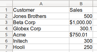
In this example, the data is a mixture of currency labeled and non-currency labeled values. For a small example like this, you might want to clean it up at the source file. However, when you have a large data set (with manually entered data), you will have no choice but to start with the messy data and clean it in pandas.
Before going further, it may be helpful to review my prior article on data types. In fact,
working on this article drove me to modify my original article to clarify the types of data
stored in
object
columns.
Let’s read in the data:
importpandasaspddf_orig=pd.read_excel('sales_cleanup.xlsx')df=df_orig.copy()| Customer | Sales | |
|---|---|---|
| 0 | Jones Brothers | 500 |
| 1 | Beta Corp | $1,000.00 |
| 2 | Globex Corp | 300.1 |
| 3 | Acme | $750.01 |
| 4 | Initech | 300 |
| 5 | Hooli | 250 |
I’ve read in the data and made a copy of it in order to preserve the original.
One of the first things I do when loading data is to check the types:
df.dtypesCustomerobjectSalesobjectdtype:objectNot surprisingly the
Sales
column is stored as an object. The ‘$’ and ‘,’ are dead giveaways
that the
Sales
column is not a numeric column. More than likely we want to do some math on the column
so let’s try to convert it to a float.
In the real world data set, you may not be so quick to see that there are non-numeric values in the
column. In my data set, my first approach was to try to use
astype()
df['Sales'].astype('float')---------------------------------------------------------------------------ValueErrorTraceback(mostrecentcalllast)<ipython-input-50-547a9c970d4a>in<module>---->1df['Sales'].astype('float').....ValueError:couldnotconvertstringtofloat:'$1,000.00'The traceback includes a
ValueError
and shows that it could not convert the $1,000.00 string
to a float. Ok. That should be easy to clean up.
Let’s try removing the ‘$’ and ‘,’ using
str.replace
:
df['Sales']=df['Sales'].str.replace(',','')df['Sales']=df['Sales'].str.replace('$','')df['Sales']0NaN11000.002NaN3750.014NaN5NaNName:Sales,dtype:objectHmm. That was not what I expected. For some reason, the string values were cleaned up
but the other values were turned into
NaN
. That’s a big problem.
To be honest, this is exactly what happened to me and I spent way more time than I should have trying to figure out what was going wrong. I eventually figured it out and will walk through the issue here so you can learn from my struggles!
The twitter thread from Ted Petrou and comment from Matt Harrison summarized my issue and identified some useful pandas snippets that I will describe below.
Basically, I assumed that an
object
column contained all strings. In reality, an object column can contain
a mixture of multiple types.
Let’s look at the types in this data set.
df=df_orig.copy()df['Sales'].apply(type)0<class 'int'>
1<class 'str'>
2<class 'float'>
3<class 'str'>
4<class 'int'>
5<class 'int'>
Name: Sales, dtype: object
Ahhh. This nicely shows the issue. The
apply(type)
code runs the
type
function
on each value in the column. As you can see, some of the values are floats,
some are integers and some are strings. Overall, the column
dtype
is an object.
Here are two helpful tips, I’m adding to my toolbox (thanks to Ted and Matt) to spot these issues earlier in my analysis process.
First, we can add a formatted column that shows each type:
df['Sales_Type']=df['Sales'].apply(lambdax:type(x).__name__)| Customer | Sales | Sales_Type | |
|---|---|---|---|
| 0 | Jones Brothers | 500 | int |
| 1 | Beta Corp | $1,000.00 | str |
| 2 | Globex Corp | 300.1 | float |
| 3 | Acme | $750.01 | str |
| 4 | Initech | 300 | int |
| 5 | Hooli | 250 | int |
Or, here is a more compact way to check the types of data in a column using
value_counts()
:
df['Sales'].apply(type).value_counts()<class 'int'> 3<class 'str'> 2<class 'float'> 1
Name: Sales, dtype: int64
I will definitely be using this in my day to day analysis when dealing with mixed data types.
Fixing the Problem
To illustrate the problem, and build the solution; I will show a quick example of a similar problem using only python data types.
First, build a numeric and string variable.
number=1235number_string='$1,235'print(type(number_string),type(number))<class 'str'> <class 'int'>
This example is similar to our data in that we have a string and an integer. If we want to clean up the string to remove the extra characters and convert to a float:
float(number_string.replace(',','').replace('$',''))1235.0Ok. That’s what we want.
What happens if we try the same thing to our integer?
float(number.replace(',','').replace('$',''))---------------------------------------------------------------------------AttributeErrorTraceback(mostrecentcalllast)<ipython-input-66-fe0f3ed32c3e>in<module>---->1float(number.replace(',','').replace('$',''))AttributeError:'int'objecthasnoattribute'replace'There’s the problem. We get an error trying to use string functions on an integer.
When pandas tries to do a similar approach by using the
str
accessor, it returns an
NaN
instead of an error. That’s why the numeric values get converted to
NaN
.
The solution is to check if the value is a string, then try to clean it up. Otherwise, avoid calling string functions on a number.
The first approach is to write a custom function and use
apply
.
defclean_currency(x):""" If the value is a string, then remove currency symbol and delimiters otherwise, the value is numeric and can be converted"""ifisinstance(x,str):return(x.replace('$','').replace(',',''))return(x)This function will check if the supplied value is a string and if it is, will remove all the characters we don’t need. If it is not a string, then it will return the original value.
Here is how we call it and convert the results to a float. I also show the column with the types:
df['Sales']=df['Sales'].apply(clean_currency).astype('float')df['Sales_Type']=df['Sales'].apply(lambdax:type(x).__name__)| Customer | Sales | Sales_Type | |
|---|---|---|---|
| 0 | Jones Brothers | 500.00 | float |
| 1 | Beta Corp | 1000.00 | float |
| 2 | Globex Corp | 300.10 | float |
| 3 | Acme | 750.01 | float |
| 4 | Initech | 300.00 | float |
| 5 | Hooli | 250.00 | float |
We can also check the
dtypes
:
df.dtypesCustomerobjectSalesfloat64Sales_Typeobjectdtype:objectOr look at the
value_counts
:
df['Sales'].apply(type).value_counts()<class 'float'> 6
Name: Sales, dtype: int64
Ok. That all looks good. We can proceed with any mathematical functions we need to apply on the sales column.
Before finishing up, I’ll show a final example of how this can be accomplished using a lambda function:
df=df_orig.copy()df['Sales']=df['Sales'].apply(lambdax:x.replace('$','').replace(',','')ifisinstance(x,str)elsex).astype(float)The lambda function is a more compact way to clean and convert the value but might be more difficult for new users to understand. I personally like a custom function in this instance. Especially if you have to clean up multiple columns.
The final caveat I have is that you still need to understand your data before doing this cleanup. I am assuming that all of the sales values are in dollars. That may or may not be a valid assumption.
If there are mixed currency values here, then you will need to develop a more complex cleaning approach to convert to a consistent numeric format. Pyjanitor has a function that can do currency conversions and might be a useful solution for more complex problems.
Summary
The pandas
object
data type is commonly used to store strings. However, you
can not assume that the data types in a column of pandas
objects
will all be strings.
This can be especially confusing when loading messy currency data that might include numeric values
with symbols as well as integers and floats.
It is quite possible that naive cleaning approaches will inadvertently convert numeric values to
NaN
.
This article shows how to use a couple of pandas tricks to identify the individual types in an object
column, clean them and convert them to the appropriate numeric value.
I hope you have found this useful. If you have any other tips or questions, let me know in the comments.
↧