Quantcast
Channel: Planet Python
Viewing all 22869 articles
Browse latest View live

PyCoder’s Weekly: Issue #383 (Aug. 27, 2019)

$
0
0

#383 – AUGUST 27, 2019
View in Browser »

The PyCoder’s Weekly Logo


Your Guide to the CPython Source Code

In this detailed Python tutorial, you’ll explore the CPython source code. By following this step-by-step walkthrough, you’ll take a deep dive into how the CPython compiler works and how your Python code gets executed.
REAL PYTHON

Refactoring Functions to Multiple Exit Points

“It’s sometimes claimed that not only should a function have a single entry point, but that it should also have a single exit. One could argue such from sense of mathematical purity. But unless you work in a programming language that combines mathematical purity with convenience […] that point seems moot to me.”
MARTIJN FAASSEN

Safely Roll Out New Features in Python With Optimizely Rollouts

alt

Tired of code rollbacks, hotfixes, or merge conflicts? Instantly turn on or off features in production. Comes with unlimited collaborators and feature flags. Embrace safer CI/CD releases with SDKs for Python and all major platforms. Get started today for free →
OPTIMIZELYsponsor

Python 3 Readiness Update

This is an automated Python 3 support table for the most popular packages. 360 out of the 360 most downloaded packages on PyPI now support Python 3.
PY3READINESS.ORG

Time to Shed Python 2

“Don’t constrict yourself, Python 2 slithers off into the sunset in 2020.”
NCSC.GOV.UK

Discussions

Python Jobs

Python Web Developer (Remote)

Premiere Digital Services

Senior Backend Software Engineer (Remote)

Close

Senior Python Developer (Austin, TX)

InQuest

Backend and DataScience Engineers (London, Relocation & Visa Possible)

Citymapper Ltd

Software Engineering Lead, Python (Houston, TX)

SimpleLegal

Software Engineer (Multiple US Locations)

Invitae

Senior Software Developer (Edmonton, AB)

Levven Electronics Ltd.

Lead Data Scientist (Buffalo, NY)

Utilant LLC

More Python Jobs >>>

Articles & Tutorials

How to Use Python Lambda Functions

Learn about Python lambda functions and see how they compare with regular functions and how you can use them in accordance with best practices.
REAL PYTHONvideo

Quick and Dirty Mock Service With Starlette

“Have you ever needed to mock out a third party service for use in a large testing environment? I recently did, and I used Starlette, a new async Python web framework, to do it. See what Starlette offers!”
MATT LAYMAN• Shared by Matt Layman

Python Developers Are in Demand on Vettery

alt

Vettery is an online hiring marketplace that’s changing the way people hire and get hired. Ready for a bold career move? Make a free profile, name your salary, and connect with hiring managers from top employers today →
VETTERYsponsor

Insider Trading Visualized With Python

“We use Python to visualize insider trading as reporting in SEC Form 4 filings. Our goal is find patterns to create signals for buy/sell decisions and general risk monitoring of investment portfolios.”
JAN L. SCHROEDER

Editing Excel Spreadsheets in Python With openpyxl

Learn how to handle spreadsheets in Python using the openpyxl package. You’ll see how to manipulate Excel spreadsheets, extract information from spreadsheets, create simple or more complex spreadsheets, including adding styles, charts, and so on.
REAL PYTHON

Handling Imbalanced Datasets With SMOTE in Python

Use SMOTE and the Python package, imbalanced-learn, to bring harmony to an imbalanced dataset.
JUAN DE DIOS SANTOS

Building an Image Hashing Search Engine With VP-Trees and OpenCV

Learn how to build a scalable image hashing search engine using OpenCV, Python, and VP-Trees.
ADRIAN ROSEBROCK

How the Gunicorn WSGI Server Works

An overview of how the Gunicorn WSGI HTTP server works internally.
REBECA SARAI

Left-Recursive PEG Grammars

Part 5 of Guido’s series on PEG parsers.
GUIDO VAN ROSSUM

Projects & Code

Events

PyCon Latam 2019

August 29 to September 1, 2019
PYLATAM.ORG

EuroSciPy 2019

September 2 to September 7, 2019
EUROSCIPY.ORG


Happy Pythoning!
This was PyCoder’s Weekly Issue #383.
View in Browser »

alt

[ Subscribe to 🐍 PyCoder’s Weekly 💌 – Get the best Python news, articles, and tutorials delivered to your inbox once a week >> Click here to learn more ]


Kushal Das: Running Ubiquity controller on a Raspberry Pi

$
0
0

I got a few new Raspberry Pi(s) with 4GB RAM. I used them as a full scale desktop for some time, and was happy with the performance.

I used to run the Ubiquity controller for the home network in a full-size desktop. Looking at the performance of this RPI model, I thought of moving it out to this machine.

I am using Debian Buster based image here. The first step is to create a new source list file at /etc/apt/sources.list.d/ubnt.list

deb https://www.ubnt.com/downloads/unifi/debian unifi5 ubiquiti

Then, install the software, and also openjdk-8-jdk, remember that the controller works only with that particular version of Java.

apt-get update
apt-get install openjdk-8-jdk unifi

We will also have to update the JAVE_HOME variable in /usr/lib/unifi/bin/unifi.init file.

JAVA_HOME=/usr/lib/jvm/java-8-openjdk-armhf/

Then, we can enable and start the service.

systemctl enable unifi
systemctl start unifi

Wingware Blog: Dark Mode and Color Configuration in Wing Python IDE

$
0
0

Wing 7 added four new dark color palettes and the ability to quickly toggle between light and dark mode using the menuicon menu icon in the top right of the IDE window. When DarkMode is selected, Wing switches to the most recently used dark color configuration, or the default dark configuration if none has been used.

To select which dark mode is used, change ColorPalette on the first page of Wing's Preferences. The dark palettes that ship with Wing 7 are:

/images/blog/dark-mode/black-background.png

Black Background: The classic original dark mode for Wing

/images/blog/dark-mode/cherry-blossom.png

Cherry Blossom: New in Wing 7

/images/blog/dark-mode/dracula.png

Dracula: New in Wing 7

/images/blog/dark-mode/monokai.png

Monokai

/images/blog/dark-mode/one-dark.png

One Dark: The default dark color palette

/images/blog/dark-mode/positronic.png

Positronic: New in Wing 7

/images/blog/dark-mode/solarized-dark.png

Solarized Dark

/images/blog/dark-mode/sun-steel.png

Sun Steel: New in Wing 7

In most cases you will also want to enable the UserInterface>UseColorPaletteThroughouttheUI preference, so that the color palette is applied to more than just editors. This preference is enabled automatically when the DarkMode menu item is used for the first time, and is enabled in all of the above screenshots. However, it may be disabled so only the editors are displayed dark. Wing will remember that choice when subsequently changing between light and dark modes.

Note that on macOS 10.14+ with Wing 7.1+, the system-defined Dark Mode may be used instead, by leaving the UserInterface>UseColorPaletteThroughouttheUI preference unchecked, and then selecting Dark Mode in the macOS System Preferences. In this approach, the ColorPalette preference in Wing should be set to ClassicDefault or one of the dark color palettes.

Color Configuration

Aside from selecting the overall color palette with the UserInterface>ColorPalette preference, it is also possible to override individual colors throughout the preferences, or to write your own color palette, including colors for the UI and optionally also for syntax highlighting in the editor. This is described in more detail in Display Style and Colors.


That's it for now! We'll be back soon with more Wing Tips for Wing Python IDE.

Mike Driscoll: PyDev of the Week: Katherine Kampf

$
0
0

This week we welcome Katherine Kampf (@kvkampf) as our PyDev of the Week! Katherine is a Program Manager at Microsoft, specifically for Azure Notebooks, which is Microsoft’s version of Jupyter Notebook. She also recently gave a talk at EuroPython 2019. Let’s take a few moments getting to know Katherine better!

Can you tell us a little about yourself (hobbies, education, etc):

Sure! I am currently a Program Manager for Azure Notebooks at Microsoft. I joined the company in 2017 and started working on the Big Data team. After some time there, I decided to move closer towards notebooks and Python which led me to the Python Tools team which has been a blast.

Before starting at Microsoft, I graduated from the University in Michigan where I studied Computer Science. I also grew up Ohio so the Midwest was home for quite a while and will always have my heart. While at UofM, I was also lucky enough to TA our introductory computer science course which covered both C++ and Python. I loved helping folks learn new concepts, and I’m so glad I get to continue this in some form by speaking at conferences!

Nowadays, I’m based in Seattle and love living the stereotypical Pacific Northwest life. I tend to spend my weekends skiing in the winter and hiking in summer. In between those, I love to travel around and am working on visiting all the U.S. National Parks! I’m also a dog-enthusiast and am always working on being friends’ go-to dog sitter 😊

Why did you start using Python?

I had played around with Python when I was first learning to program around 7 years ago, but I started using it on the regular around 4 years ago for an AI course at university

What other programming languages do you know and which is your favorite?

C++ is my other primary language, and it used to be my favorite, but Python has definitely stolen my heart over the past few years.

What projects are you working on now?

In my free time, I’ve been working on analyzing allll the data from the past ~5 years of wearing my Fitbit. It’s really cool to see my sleep patterns for so long as well as my general fitness habits. Hoping to see some interesting trends by looking at my exercise in relation to sleep and weather. We’ll see! I’m also working on building a Porta Pi mini arcade machine which I’m super excited about.

And in my job, I’m working on making Azure Notebooks the most productive experience for notebooks-users 😊

Which Python libraries are your favorite (core or 3rd party)?

I will always love NLTK! I was exposed to it early on in my Python career and found it so powerful. And still do! Natural language has always been super interesting to me and I love all NLTK helps with!

Is there anything else you’d like to say?

I always encourage folks to share their knowledge in whatever ways they can! And to overcome the imposter syndrome that comes with it.

Thanks for doing the interview, Katherine!

The post PyDev of the Week: Katherine Kampf appeared first on The Mouse Vs. The Python.

IslandT: Capitalize the letters that occupy even indexes and odd indexes separately

$
0
0

Given a string, capitalize the letters within the string that occupy even indexes and odd indexes separately, and return as a list! Index 0 will be considered even.

For example, capitalize(“abcdef”) = [‘AbCdEf’, ‘aBcDeF’]!

The input will be a lowercase string with no spaces.

def capitalize(s):
    s = list(s)
    li = []
    stri = ''
    n = 1
    first = False
    time = 0
    while(time < 2):

        if first == False:
            for e in s:
                if n % 2 != 0:
                    stri += e.upper()
                else:
                    stri += e
                n+=1
            first = True
            n = 1
            li.append(stri)
            stri = ''
            time += 1
        else:
            for e in s:
                if n % 2 == 0:
                    stri += e.upper()
                else:
                    stri += e
                n+=1
            li.append(stri)
            time += 1
    return li

Do you know we actually can achieve the above outcome with just 3 lines of code? Provide your answer in the comment box below!

Django Weblog: Django bugfix releases issued: 2.2.5, 2.1.12, and 1.11.24

$
0
0

Today we've issued 2.2.5, 2.1.12, and 1.11.24 bugfix releases.

The release package and checksums are available from our downloads page, as well as from the Python Package Index. The PGP key ID used for this release is Mariusz Felisiak: 2EF56372BA48CD1B.

PyBites: Code Challenge 63 - Automatically Generate Blog Featured Images

$
0
0

There is an immense amount to be learned simply by tinkering with things. - Henry Ford

Hey Pythonistas,

In this new blog code challenge you are going to use selenium to automatically generate some cool featured images for PyBites. Let's write some Python code, shall we?

The Challenge

Some time ago Bob made a tool to automate blog image generation: Featured Image Creator.

In this challenge you will help PyBites create some nice featured images for their code challenges or articles (heck, we could even use them on Twitter!)

Steps:

  1. Make a virtual env and pip install selenium (and optionally bs4 or feedparser), however this is not a requirement, use your favorite tools ...

  2. Scrape all blog code challenge titles and/or PyBites articles (feel free to feedparse our RSS feed). We want images for all of them.

  3. Using Selenium navigate to Featured Image Creator and set the canvas (button ID #submitDimensions) to your preferred size (e.g. w=300/ h=100, or w=200 / h=200)

  4. Loop over the challenge and/or article titles you scraped and for each title:

    • enter the title alongside Title text in image (blog post) (#title ID field).

    • choose a Margin-top and Google Font from the two dropdown fields (#topoffset and #font field IDs respectively).

    • choose a theme: BG theme: material or BG theme: bamboo (#collection ID field).

    • choose a picture from the auto-complete (#bg1_url ID field), or just fill in the field picking random ones from the 2 lists below (one per theme):

      featured_image/images/material]# ls -C1|grep full|sort|sed 's@\(.*\)@images/material/\1@g'
      images/material/black-blue_full.jpg
      images/material/black_full.jpg
      images/material/black-red_full.jpg
      images/material/blue-black_full.jpg
      images/material/blue-brown_full.png
      images/material/blue_full.jpg
      images/material/blue-green_full.png
      images/material/blue-lightblue-white_full.jpg
      images/material/blue-white_full.jpg
      images/material/blue-yellow_full.png
      images/material/darkgreen-red-yellow_full.png
      images/material/green-blue_full.jpg
      images/material/green_full.png
      images/material/green-red_full.jpg
      images/material/orange-black_full.jpg
      images/material/orange-blue_full.jpg
      images/material/purple-blue_full.jpg
      images/material/purple-blue-red_full.jpg
      images/material/purple-red-orange_full.png
      images/material/purple-red-white_full.png
      images/material/purple-yellow-white_full.png
      images/material/red_full.jpg
      images/material/red-green_full.jpg
      images/material/white-blue_full.png
      images/material/yellow-darkgrey-red_full.jpg
      
      featured_image/images/bamboo]# ls -C1|grep full|sort -n|sed 's@\(.*\)@images/bamboo/\1@g'
      images/bamboo/1_green_full.jpg
      images/bamboo/2_black_full.jpg
      images/bamboo/3_black_full.jpg
      images/bamboo/4_black_full.jpg
      images/bamboo/5_black_full.jpg
      images/bamboo/6_white_black_full.jpg
      images/bamboo/7_black_full.jpg
      images/bamboo/8_black_full.jpg
      images/bamboo/9_black_full.jpg
      images/bamboo/10_green_full.jpg
      images/bamboo/11_black_full.jpg
      images/bamboo/12_black_olive_full.jpg
      images/bamboo/13_gray_full.jpg
      images/bamboo/14_black_full.jpg
      images/bamboo/15_green_full.jpg
      images/bamboo/16_black_full.jpg
      images/bamboo/17_green_white_olive_full.jpg
      images/bamboo/18_black_full.jpg
      images/bamboo/19_green_full.jpg
      images/bamboo/20_gray_full.jpg
      images/bamboo/21_silver_full.jpg
      images/bamboo/22_white_full.jpg
      images/bamboo/23_black_olive_full.jpg
      images/bamboo/24_white_full.jpg
      images/bamboo/25_black_white_full.jpg
      
  5. Feel free to set the other fields as well, but so far your should have a decent featured image, so move onto to saving the image ...

  6. Click the Save button (#btnSave ID field).

  7. Move the obtained file to an output directory and zip them up (using Python's zipfile).

PR your work on our platform including the generated zipfile (or host it yourself and link in the PR to keep our challenges repo lean).

Good luck and have fun coding Python! Ideas for future challenges? use GH Issues.


Get serious, take your Python to the next level ...

At PyBites we're all about creating Python ninjas through challenges and real-world exercises. Read more about our story.

We are happy and proud to share that we now hear monthly stories from our users that they're landing new Python jobs. For many this is a dream come true, especially as they're often landing roles with significantly higher salaries!

Our 200 Bites of Py exercises are geared toward instilling the habit of coding frequently, if not daily which will dramatically improve your Python and problem solving skills. This is THE number one skillset necessary to becoming a linchpin in the industry and will enable you to crush it wherever codes need to be written.

Take our free trial and let us know on Slack how it helps you improve your Python!


>>>frompybitesimportBob,JulianKeepCalmandCodeinPython!

Julien Danjou: Dependencies Handling in Python

$
0
0
Dependencies Handling in Python

Dependencies are a nightmare for many people. Some even argue they are technical debt. Managing the list of the libraries of your software is a horrible experience. Updating them — automatically? — sounds like a delirium.

Stick with me here as I am going to help you get a better grasp on something that you cannot, in practice, get rid of — unless you're incredibly rich and talented and can live without the code of others.

First, we need to be clear of something about dependencies: there are two types of them. Donald Stuff wrote better than I would about the subject years ago. To make it simple, one can say that they are two types of code packages depending on  external code: applications and libraries.

Libraries Dependencies

Python libraries should specify their dependencies in a generic way. A library should not require requests 2.1.5: it does not make sense. If every library out there needs a different version of requests, they can't be used at the same time.

Libraries need to declare dependencies based on ranges of version numbers. Requiring requests>=2 is correct. Requiring requests>=1,<2 is also correct if you know that requests 2.x does not work with the library. The problem that your version range specification is solving is the API compatibility issue between your code and your dependencies — nothing else. That's a good reason for libraries to use Semantic Versioning whenever possible.

Therefore, dependencies should be written in setup.py as something like:

from setuptools import setup

setup(
    name="MyLibrary",
    version="1.0",
    install_requires=[
        "requests",
    ],
    # ...
)

This way, it is easy for any application to use the library and co-exist with others.

Applications Dependencies

An application is just a particular case of libraries. They are not intended to be reused (imported) by other libraries of applications — though nothing would prevent it in practice.

In the end, that means that you should specify the dependencies the same way that you would do for a library in the application's setup.py.

The main difference is that an application is usually deployed in production to provide its service. Deployments need to be reproducible. For that, you can't solely rely on setup.py: the requested range of the dependencies are too broad. You're at the mercy of random version changes at any time when re-deploying your application.

You, therefore, need a different version management mechanism to handle deployment than just setup.py.

pipenv has an excellent section recapping this in its documentation. It splits dependency types into abstract and concrete dependencies: abstract dependencies are based on ranges (e.g., libraries) whereas concrete dependencies are specified with precise versions (e.g., application deployments) — as we've just seen here.

Handling Deployment

The requirements.txt file has been used to solve application deployment reproducibility for a long time now. Its format is usually something like:

requests==3.1.5
foobar==2.0

Each library sees itself specified to the micro version. That makes sure each of your deployment is going to install the same version of your dependency. Using a requirements.txt is a simple solution and a first step toward reproducible deployment. However, it's not enough.

Indeed, while you can specify which version of requests you with, it requests depends on urllib3 and that could make pip install urllib 2.1 or urllib 2.2. You can't know, which does not make your deployment 100% reproducible.

Of course, you could duplicate all requests dependencies yourself in your requirements.txt, but that would be madness!

Dependencies Handling in PythonAn application dependency tree can be quite deep and complex sometimes.

There are various hacks available to fix this limitation, but the real saviors here are pipenv and poetry. The way they solve it is similar to many package managers in other programming languages. They generate a lock file that contains the list of all installed dependencies (and their own dependencies, etc.) with their version numbers. That makes sure the deployment is 100% reproducible.

Check out their documentation on how to set up and use them!

Handling Dependencies Updates

Now that you have your lock file that makes sure your deployment is reproducible in a snap, you've another problem. How do you make sure that your dependencies are up-to-date? There is a real security concern about this, but also bug fixes and optimizations that you might miss by staying behind.

If your project is hosted on GitHub, Dependabot is an excellent solution to solve this issue. Enabling this application on your repository creates automatically pull requests whenever a new version of the library listed in your lock file is available. For example, if you've deployed your application with redis 3.3.6, Dependabot will create a pull request updating to redis 3.3.7 as soon as it gets released. Furthermore, Dependabot supports requirements.txt, pipenv, and poetry!

Dependencies Handling in PythonDependabot updating jinja2 for you

Automatic Deployment Update

You're almost there. You have a bot that is letting you know that a new version of a library your project needs is available.

Once the pull request is created, your continuous integration system is going to kick in, deploy your project, and runs the test. If everything works fine, your pull request is ready to be merged. But are you really needed in this process?

Unless you have a particular and personal aversion on specific version numbers —"Gosh I hate versions that end with a 3. It's always bad luck."— or unless you have zero automated testing, you, human, is useless. This merge can be fully automatic.

This is where Mergify comes into play. Mergify is a GitHub application allowing to define precise rules about how to merge your pull requests. Here's a rule that I use in every project:

pull_requests_rules:
  - name: automatic merge from dependabot
    conditions:
      - author~=^dependabot(|-preview)\[bot\]$
      - label!=work-in-progress
      - "status-success=ci/circleci: pep8"
      - "status-success=ci/circleci: py37"
    actions:
      merge:
        method: merge
Dependencies Handling in PythonMergify reports when the rule fully matches

As soon as your continuous integration system passes, Mergify merges the pull request for you.

Dependencies Handling in Python

You can then automatically trigger your deployment hooks to update your production deployment and get the new library version installed right away. This leaves your application always up-to-date with newer libraries and not lagging behind several years of releases.

If anything goes wrong, you're still able to revert the commit from Dependabot — which you can also automate if you wish with a Mergify rule.

Beyond

This is to me the state of the art of dependency management lifecycle right now. And while this applies exceptionally well to Python, it can be applied to many other languages that use a similar pattern — such as Node and npm.


EuroPython: EuroPython 2019: Please send in your feedback

$
0
0

EuroPython 2019 is over now and so it’s time to ask around for what we can improve next year. If you attended EuroPython 2019, please take a few moments and fill in our feedback form, if you haven’t already done so:

image

EuroPython 2019 Feedback Form

We will leave the feedback form online for a few weeks and then use the information as basis for the work on EuroPython 2020 and also intend to post a summary of the multiple choice questions (not the comments to protect your privacy) on our website.

Many thanks in advance.

Enjoy,

EuroPython 2019 Team
https://ep2019.europython.eu/
https://www.europython-society.org/

Reuven Lerner: Reminder: Only one day left for early-bird pricing on Weekly Python Exercise A3 (objects for beginners)

$
0
0

The biggest problem with software today isn’t writing code. It’s maintaining — debugging, improving, and expanding — existing code. It’s hard to maintain someone else’s code. Heck, it’s even hard to maintain your own code. (Who among us hasn’t looked at code and said, “Who was the idiot who wrote this… oh, it was me…”?)

There’s no magic formula that’ll make code maintenance easy. But you can make it easier if (1) everyone agrees on some conventions for how the code will look and act, and (2) if you can reuse existing code, and thus write less of it.

That’s the promise of object-oriented programming: By reusing existing code, you can write less. Moreover, by agreeing to some general conventions, the code that you do write becomes easier to write and easier to read — and thus, easier to maintain.

Sounds great, right? It is, but (of course) there’s a catch: Object-oriented programming has a whole bunch of vocabulary, conventions, and expectations that tend to overwhelm many experienced developers with a background in objects.

And even if you have experience with objects, then Python’s way of doing things might strike you as as bit odd.

In either case, I have a solution for you: Weekly Python Exercise.

If you feel stuck with Python objects, then Weekly Python Exercise A3 (objects for beginners) is for you. We’ll cover such topics as objects, classes, instances, methods, attributes, and inheritance — not with dry lectures, but by actually solving new problems each week. Here’s how it works:

  • Every Tuesday, you’ll receive a problem description, along with some sources to read and “pytests” tests
  • On the following Monday, you’ll receive a detailed solution and explaination
  • In between, you’ll be able to participate in our exclusive forum
  • About once a month, you can join live office hours, to ask me questions and/or review the answers.

After fifteen weeks of working with objects, you’ll know how to write them, but will also understand the ideas behind them. You won’t be stuck any more, checking Stack Overflow a dozen times each day to double-check the syntax for working with objects in Python. Moreover, you’ll see the Pythonic way of doing things, helping you to write code in a way that Python developers aim to achieve.

Hundreds of developers from around the world have already enjoyed Weekly Python Exercise since it started several years ago. WPE A3 (objects for beginners) starts on September 17th, but early-bird pricing for that cohort ends tomorrow, Tuesday, September 3rd.

Questions or comments? Or think that you’re eligible for one of the many discount coupons? Read more at https://WeeklyPythonExercise.com/, or just e-mail me at reuven@lerner.co.il.

The post Reminder: Only one day left for early-bird pricing on Weekly Python Exercise A3 (objects for beginners) appeared first on Reuven Lerner.

Real Python: Natural Language Processing With spaCy in Python

$
0
0

spaCy is a free and open-source library for Natural Language Processing (NLP) in Python with a lot of in-built capabilities. It’s becoming increasingly popular for processing and analyzing data in NLP. Unstructured textual data is produced at a large scale, and it’s important to process and derive insights from unstructured data. To do that, you need to represent the data in a format that can be understood by computers. NLP can help you do that.

In this tutorial, you’ll learn:

  • What the foundational terms and concepts in NLP are
  • How to implement those concepts in spaCy
  • How to customize and extend built-in functionalities in spaCy
  • How to perform basic statistical analysis on a text
  • How to create a pipeline to process unstructured text
  • How to parse a sentence and extract meaningful insights from it

Free Bonus:Click here to get access to a chapter from Python Tricks: The Book that shows you Python's best practices with simple examples you can apply instantly to write more beautiful + Pythonic code.

What Are NLP and spaCy?

NLP is a subfield of Artificial Intelligence and is concerned with interactions between computers and human languages. NLP is the process of analyzing, understanding, and deriving meaning from human languages for computers.

NLP helps you extract insights from unstructured text and has several use cases, such as:

spaCy is a free, open-source library for NLP in Python. It’s written in Cython and is designed to build information extraction or natural language understanding systems. It’s built for production use and provides a concise and user-friendly API.

Installation

In this section, you’ll install spaCy and then download data and models for the English language.

How to Install spaCy

spaCy can be installed using pip, a Python package manager. You can use a virtual environment to avoid depending on system-wide packages. To learn more about virtual environments and pip, check out What Is Pip? A Guide for New Pythonistas and Python Virtual Environments: A Primer.

Create a new virtual environment:

$ python3 -m venv env

Activate this virtual environment and install spaCy:

$source ./env/bin/activate
$ pip install spacy

How to Download Models and Data

spaCy has different types of models. The default model for the English language is en_core_web_sm.

Activate the virtual environment created in the previous step and download models and data for the English language:

$ python -m spacy download en_core_web_sm

Verify if the download was successful or not by loading it:

>>>
>>> importspacy>>> nlp=spacy.load('en_core_web_sm')

If the nlp object is created, then it means that spaCy was installed and that models and data were successfully downloaded.

Using spaCy

In this section, you’ll use spaCy for a given input string and a text file. Load the language model instance in spaCy:

>>>
>>> importspacy>>> nlp=spacy.load('en_core_web_sm')

Here, the nlp object is a language model instance. You can assume that, throughout this tutorial, nlp refers to the language model loaded by en_core_web_sm. Now you can use spaCy to read a string or a text file.

How to Read a String

You can use spaCy to create a processed Doc object, which is a container for accessing linguistic annotations, for a given input string:

>>>
>>> introduction_text=('This tutorial is about Natural'... ' Language Processing in Spacy.')>>> introduction_doc=nlp(introduction_text)>>> # Extract tokens for the given doc>>> print([token.textfortokeninintroduction_doc])['This', 'tutorial', 'is', 'about', 'Natural', 'Language','Processing', 'in', 'Spacy', '.']

In the above example, notice how the text is converted to an object that is understood by spaCy. You can use this method to convert any text into a processed Doc object and deduce attributes, which will be covered in the coming sections.

How to Read a Text File

In this section, you’ll create a processed Doc object for a text file:

>>>
>>> file_name='introduction.txt'>>> introduction_file_text=open(file_name).read()>>> introduction_file_doc=nlp(introduction_file_text)>>> # Extract tokens for the given doc>>> print([token.textfortokeninintroduction_file_doc])['This', 'tutorial', 'is', 'about', 'Natural', 'Language','Processing', 'in', 'Spacy', '.', '\n']

This is how you can convert a text file into a processed Doc object.

Note:

You can assume that:

  • Variable names ending with the suffix _text are Unicode string objects.
  • Variable name ending with the suffix _doc are spaCy’s language model objects.

Sentence Detection

Sentence Detection is the process of locating the start and end of sentences in a given text. This allows you to you divide a text into linguistically meaningful units. You’ll use these units when you’re processing your text to perform tasks such as part of speech tagging and entity extraction.

In spaCy, the sents property is used to extract sentences. Here’s how you would extract the total number of sentences and the sentences for a given input text:

>>>
>>> about_text=('Gus Proto is a Python developer currently'... ' working for a London-based Fintech'... ' company. He is interested in learning'... ' Natural Language Processing.')>>> about_doc=nlp(about_text)>>> sentences=list(about_doc.sents)>>> len(sentences)2>>> forsentenceinsentences:... print(sentence)...'Gus Proto is a Python developer currently working for aLondon-based Fintech company.''He is interested in learning Natural Language Processing.'

In the above example, spaCy is correctly able to identify sentences in the English language, using a full stop(.) as the sentence delimiter. You can also customize the sentence detection to detect sentences on custom delimiters.

Here’s an example, where an ellipsis(...) is used as the delimiter:

>>>
>>> defset_custom_boundaries(doc):... # Adds support to use `...` as the delimiter for sentence detection... fortokenindoc[:-1]:... iftoken.text=='...':... doc[token.i+1].is_sent_start=True... returndoc...>>> ellipsis_text=('Gus, can you, ... never mind, I forgot'... ' what I was saying. So, do you think'... ' we should ...')>>> # Load a new model instance>>> custom_nlp=spacy.load('en_core_web_sm')>>> custom_nlp.add_pipe(set_custom_boundaries,before='parser')>>> custom_ellipsis_doc=custom_nlp(ellipsis_text)>>> custom_ellipsis_sentences=list(custom_ellipsis_doc.sents)>>> forsentenceincustom_ellipsis_sentences:... print(sentence)...Gus, can you, ...never mind, I forgot what I was saying.So, do you think we should ...>>> # Sentence Detection with no customization>>> ellipsis_doc=nlp(ellipsis_text)>>> ellipsis_sentences=list(ellipsis_doc.sents)>>> forsentenceinellipsis_sentences:... print(sentence)...Gus, can you, ... never mind, I forgot what I was saying.So, do you think we should ...

Note that custom_ellipsis_sentences contain three sentences, whereas ellipsis_sentences contains two sentences. These sentences are still obtained via the sents attribute, as you saw before.

Tokenization in spaCy

Tokenization is the next step after sentence detection. It allows you to identify the basic units in your text. These basic units are called tokens. Tokenization is useful because it breaks a text into meaningful units. These units are used for further analysis, like part of speech tagging.

In spaCy, you can print tokens by iterating on the Doc object:

>>>
>>> fortokeninabout_doc:... print(token,token.idx)...Gus 0Proto 4is 10a 13Python 15developer 22currently 32working 42for 50a 54London 56- 62based 63Fintech 69company 77. 84He 86is 89interested 92in 103learning 106Natural 115Language 123Processing 132. 142

Note how spaCy preserves the starting index of the tokens. It’s useful for in-place word replacement. spaCy provides various attributes for the Token class:

>>>
>>> fortokeninabout_doc:... print(token,token.idx,token.text_with_ws,... token.is_alpha,token.is_punct,token.is_space,... token.shape_,token.is_stop)...Gus 0 Gus  True False False Xxx FalseProto 4 Proto  True False False Xxxxx Falseis 10 is  True False False xx Truea 13 a  True False False x TruePython 15 Python  True False False Xxxxx Falsedeveloper 22 developer  True False False xxxx Falsecurrently 32 currently  True False False xxxx Falseworking 42 working  True False False xxxx Falsefor 50 for  True False False xxx Truea 54 a  True False False x TrueLondon 56 London True False False Xxxxx False- 62 - False True False - Falsebased 63 based  True False False xxxx FalseFintech 69 Fintech  True False False Xxxxx Falsecompany 77 company True False False xxxx False. 84 .  False True False . FalseHe 86 He  True False False Xx Trueis 89 is  True False False xx Trueinterested 92 interested  True False False xxxx Falsein 103 in  True False False xx Truelearning 106 learning  True False False xxxx FalseNatural 115 Natural  True False False Xxxxx FalseLanguage 123 Language  True False False Xxxxx FalseProcessing 132 Processing True False False Xxxxx False. 142 . False True False . False

In this example, some of the commonly required attributes are accessed:

  • text_with_ws prints token text with trailing space (if present).
  • is_alpha detects if the token consists of alphabetic characters or not.
  • is_punct detects if the token is a punctuation symbol or not.
  • is_space detects if the token is a space or not.
  • shape_ prints out the shape of the word.
  • is_stop detects if the token is a stop word or not.

Note: You’ll learn more about stop words in the next section.

You can also customize the tokenization process to detect tokens on custom characters. This is often used for hyphenated words, which are words joined with hyphen. For example, “London-based” is a hyphenated word.

spaCy allows you to customize tokenization by updating the tokenizer property on the nlp object:

>>>
>>> importre>>> importspacy>>> fromspacy.tokenizerimportTokenizer>>> custom_nlp=spacy.load('en_core_web_sm')>>> prefix_re=spacy.util.compile_prefix_regex(custom_nlp.Defaults.prefixes)>>> suffix_re=spacy.util.compile_suffix_regex(custom_nlp.Defaults.suffixes)>>> infix_re=re.compile(r'''[-~]''')>>> defcustomize_tokenizer(nlp):... # Adds support to use `-` as the delimiter for tokenization... returnTokenizer(nlp.vocab,prefix_search=prefix_re.search,... suffix_search=suffix_re.search,... infix_finditer=infix_re.finditer,... token_match=None... )...>>> custom_nlp.tokenizer=customize_tokenizer(custom_nlp)>>> custom_tokenizer_about_doc=custom_nlp(about_text)>>> print([token.textfortokenincustom_tokenizer_about_doc])['Gus', 'Proto', 'is', 'a', 'Python', 'developer', 'currently','working', 'for', 'a', 'London', '-', 'based', 'Fintech','company', '.', 'He', 'is', 'interested', 'in', 'learning','Natural', 'Language', 'Processing', '.']

In order for you to customize, you can pass various parameters to the Tokenizer class:

  • nlp.vocab is a storage container for special cases and is used to handle cases like contractions and emoticons.
  • prefix_search is the function that is used to handle preceding punctuation, such as opening parentheses.
  • infix_finditer is the function that is used to handle non-whitespace separators, such as hyphens.
  • suffix_search is the function that is used to handle succeeding punctuation, such as closing parentheses.
  • token_match is an optional boolean function that is used to match strings that should never be split. It overrides the previous rules and is useful for entities like URLs or numbers.

Note: spaCy already detects hyphenated words as individual tokens. The above code is just an example to show how tokenization can be customized. It can be used for any other character.

Stop Words

Stop words are the most common words in a language. In the English language, some examples of stop words are the, are, but, and they. Most sentences need to contain stop words in order to be full sentences that make sense.

Generally, stop words are removed because they aren’t significant and distort the word frequency analysis. spaCy has a list of stop words for the English language:

>>>
>>> importspacy>>> spacy_stopwords=spacy.lang.en.stop_words.STOP_WORDS>>> len(spacy_stopwords)326>>> forstop_wordinlist(spacy_stopwords)[:10]:... print(stop_word)...usingbecomeshaditselfonceoftenishereinwhotoo

You can remove stop words from the input text:

>>>
>>> fortokeninabout_doc:... ifnottoken.is_stop:... print(token)...GusProtoPythondevelopercurrentlyworkingLondon-basedFintechcompany.interestedlearningNaturalLanguageProcessing.

Stop words like is, a, for, the, and in are not printed in the output above. You can also create a list of tokens not containing stop words:

>>>
>>> about_no_stopword_doc=[tokenfortokeninabout_docifnottoken.is_stop]>>> print(about_no_stopword_doc)[Gus, Proto, Python, developer, currently, working, London,-, based, Fintech, company, ., interested, learning, Natural,Language, Processing, .]

about_no_stopword_doc can be joined with spaces to form a sentence with no stop words.

Lemmatization

Lemmatization is the process of reducing inflected forms of a word while still ensuring that the reduced form belongs to the language. This reduced form or root word is called a lemma.

For example, organizes, organized and organizing are all forms of organize. Here, organize is the lemma. The inflection of a word allows you to express different grammatical categories like tense (organized vs organize), number (trains vs train), and so on. Lemmatization is necessary because it helps you reduce the inflected forms of a word so that they can be analyzed as a single item. It can also help you normalize the text.

spaCy has the attribute lemma_ on the Token class. This attribute has the lemmatized form of a token:

>>>
>>> conference_help_text=('Gus is helping organize a developer'... 'conference on Applications of Natural Language'... ' Processing. He keeps organizing local Python meetups'... ' and several internal talks at his workplace.')>>> conference_help_doc=nlp(conference_help_text)>>> fortokeninconference_help_doc:... print(token,token.lemma_)...Gus Gusis behelping helporganize organizea adeveloper developerconference conferenceon onApplications Applicationsof ofNatural NaturalLanguage LanguageProcessing Processing. .He -PRON-keeps keeporganizing organizelocal localPython Pythonmeetups meetupand andseveral severalinternal internaltalks talkat athis -PRON-workplace workplace. .

In this example, organizing reduces to its lemma form organize. If you do not lemmatize the text, then organize and organizing will be counted as different tokens, even though they both have a similar meaning. Lemmatization helps you avoid duplicate words that have similar meanings.

Word Frequency

You can now convert a given text into tokens and perform statistical analysis over it. This analysis can give you various insights about word patterns, such as common words or unique words in the text:

>>>
>>> fromcollectionsimportCounter>>> complete_text=('Gus Proto is a Python developer currently'... 'working for a London-based Fintech company. He is'... ' interested in learning Natural Language Processing.'... ' There is a developer conference happening on 21 July'... ' 2019 in London. It is titled "Applications of Natural'... ' Language Processing". There is a helpline number '... ' available at +1-1234567891. Gus is helping organize it.'... ' He keeps organizing local Python meetups and several'... ' internal talks at his workplace. Gus is also presenting'... ' a talk. The talk will introduce the reader about "Use'... ' cases of Natural Language Processing in Fintech".'... ' Apart from his work, he is very passionate about music.'... ' Gus is learning to play the Piano. He has enrolled '... ' himself in the weekend batch of Great Piano Academy.'... ' Great Piano Academy is situated in Mayfair or the City'... ' of London and has world-class piano instructors.')...>>> complete_doc=nlp(complete_text)>>> # Remove stop words and punctuation symbols>>> words=[token.textfortokenincomplete_doc... ifnottoken.is_stopandnottoken.is_punct]>>> word_freq=Counter(words)>>> # 5 commonly occurring words with their frequencies>>> common_words=word_freq.most_common(5)>>> print(common_words)[('Gus', 4), ('London', 3), ('Natural', 3), ('Language', 3), ('Processing', 3)]>>> # Unique words>>> unique_words=[wordfor(word,freq)inword_freq.items()iffreq==1]>>> print(unique_words)['Proto', 'currently', 'working', 'based', 'company','interested', 'conference', 'happening', '21', 'July','2019', 'titled', 'Applications', 'helpline', 'number','available', '+1', '1234567891', 'helping', 'organize','keeps', 'organizing', 'local', 'meetups', 'internal','talks', 'workplace', 'presenting', 'introduce', 'reader','Use', 'cases', 'Apart', 'work', 'passionate', 'music', 'play','enrolled', 'weekend', 'batch', 'situated', 'Mayfair', 'City','world', 'class', 'piano', 'instructors']

By looking at the common words, you can see that the text as a whole is probably about Gus, London, or Natural Language Processing. This way, you can take any unstructured text and perform statistical analysis to know what it’s about.

Here’s another example of the same text with stop words:

>>>
>>> words_all=[token.textfortokenincomplete_docifnottoken.is_punct]>>> word_freq_all=Counter(words_all)>>> # 5 commonly occurring words with their frequencies>>> common_words_all=word_freq_all.most_common(5)>>> print(common_words_all)[('is', 10), ('a', 5), ('in', 5), ('Gus', 4), ('of', 4)]

Four out of five of the most common words are stop words, which don’t tell you much about the text. If you consider stop words while doing word frequency analysis, then you won’t be able to derive meaningful insights from the input text. This is why removing stop words is so important.

Part of Speech Tagging

Part of speech or POS is a grammatical role that explains how a particular word is used in a sentence. There are eight parts of speech:

  1. Noun
  2. Pronoun
  3. Adjective
  4. Verb
  5. Adverb
  6. Preposition
  7. Conjunction
  8. Interjection

Part of speech tagging is the process of assigning a POS tag to each token depending on its usage in the sentence. POS tags are useful for assigning a syntactic category like noun or verb to each word.

In spaCy, POS tags are available as an attribute on the Token object:

>>>
>>> fortokeninabout_doc:... print(token,token.tag_,token.pos_,spacy.explain(token.tag_))...Gus NNP PROPN noun, proper singularProto NNP PROPN noun, proper singularis VBZ VERB verb, 3rd person singular presenta DT DET determinerPython NNP PROPN noun, proper singulardeveloper NN NOUN noun, singular or masscurrently RB ADV adverbworking VBG VERB verb, gerund or present participlefor IN ADP conjunction, subordinating or prepositiona DT DET determinerLondon NNP PROPN noun, proper singular- HYPH PUNCT punctuation mark, hyphenbased VBN VERB verb, past participleFintech NNP PROPN noun, proper singularcompany NN NOUN noun, singular or mass. . PUNCT punctuation mark, sentence closerHe PRP PRON pronoun, personalis VBZ VERB verb, 3rd person singular presentinterested JJ ADJ adjectivein IN ADP conjunction, subordinating or prepositionlearning VBG VERB verb, gerund or present participleNatural NNP PROPN noun, proper singularLanguage NNP PROPN noun, proper singularProcessing NNP PROPN noun, proper singular. . PUNCT punctuation mark, sentence closer

Here, two attributes of the Token class are accessed:

  1. tag_ lists the fine-grained part of speech.
  2. pos_ lists the coarse-grained part of speech.

spacy.explain gives descriptive details about a particular POS tag. spaCy provides a complete tag list along with an explanation for each tag.

Using POS tags, you can extract a particular category of words:

>>>
>>> nouns=[]>>> adjectives=[]>>> fortokeninabout_doc:... iftoken.pos_=='NOUN':... nouns.append(token)... iftoken.pos_=='ADJ':... adjectives.append(token)...>>> nouns[developer, company]>>> adjectives[interested]

You can use this to derive insights, remove the most common nouns, or see which adjectives are used for a particular noun.

Visualization: Using displaCy

spaCy comes with a built-in visualizer called displaCy. You can use it to visualize a dependency parse or named entities in a browser or a Jupyter notebook.

You can use displaCy to find POS tags for tokens:

>>>
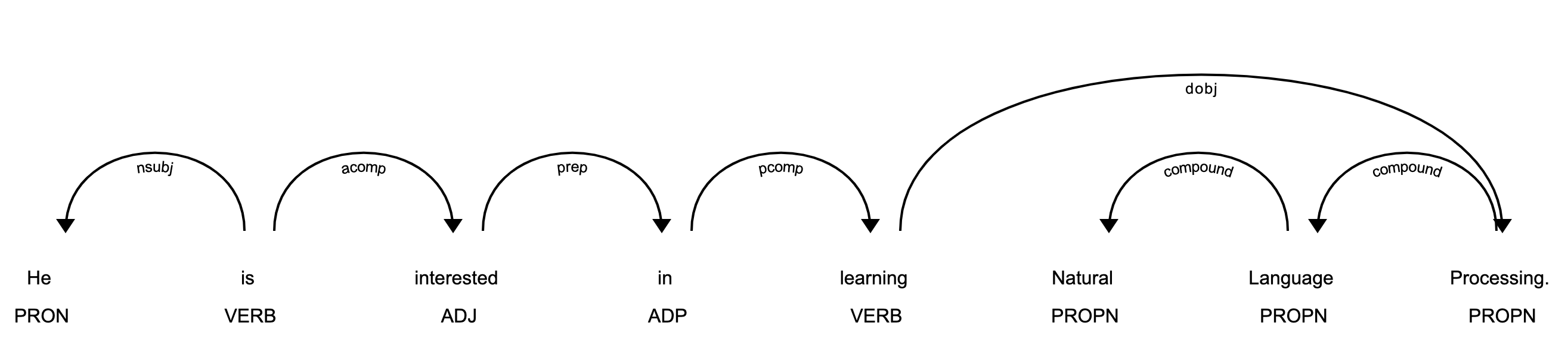
>>> fromspacyimportdisplacy>>> about_interest_text=('He is interested in learning'... ' Natural Language Processing.')>>> about_interest_doc=nlp(about_interest_text)>>> displacy.serve(about_interest_doc,style='dep')

The above code will spin a simple web server. You can see the visualization by opening http://127.0.0.1:5000 in your browser:

Displacy: Part of Speech Tagging DemodisplaCy: Part of Speech Tagging Demo

In the image above, each token is assigned a POS tag written just below the token.

Note: Here’s how you can use displaCy in a Jupyter notebook:

>>>
>>> displacy.render(about_interest_doc,style='dep',jupyter=True)

Preprocessing Functions

You can create a preprocessing function that takes text as input and applies the following operations:

  • Lowercases the text
  • Lemmatizes each token
  • Removes punctuation symbols
  • Removes stop words

A preprocessing function converts text to an analyzable format. It’s necessary for most NLP tasks. Here’s an example:

>>>
>>> defis_token_allowed(token):... '''...         Only allow valid tokens which are not stop words...         and punctuation symbols....     '''... if(nottokenornottoken.string.strip()or... token.is_stoportoken.is_punct):... returnFalse... returnTrue...>>> defpreprocess_token(token):... # Reduce token to its lowercase lemma form... returntoken.lemma_.strip().lower()...>>> complete_filtered_tokens=[preprocess_token(token)... fortokenincomplete_docifis_token_allowed(token)]>>> complete_filtered_tokens['gus', 'proto', 'python', 'developer', 'currently', 'work','london', 'base', 'fintech', 'company', 'interested', 'learn','natural', 'language', 'processing', 'developer', 'conference','happen', '21', 'july', '2019', 'london', 'title','applications', 'natural', 'language', 'processing', 'helpline','number', 'available', '+1', '1234567891', 'gus', 'help','organize', 'keep', 'organize', 'local', 'python', 'meetup','internal', 'talk', 'workplace', 'gus', 'present', 'talk', 'talk','introduce', 'reader', 'use', 'case', 'natural', 'language','processing', 'fintech', 'apart', 'work', 'passionate', 'music','gus', 'learn', 'play', 'piano', 'enrol', 'weekend', 'batch','great', 'piano', 'academy', 'great', 'piano', 'academy','situate', 'mayfair', 'city', 'london', 'world', 'class','piano', 'instructor']

Note that the complete_filtered_tokens does not contain any stop word or punctuation symbols and consists of lemmatized lowercase tokens.

Rule-Based Matching Using spaCy

Rule-based matching is one of the steps in extracting information from unstructured text. It’s used to identify and extract tokens and phrases according to patterns (such as lowercase) and grammatical features (such as part of speech).

Rule-based matching can use regular expressions to extract entities (such as phone numbers) from an unstructured text. It’s different from extracting text using regular expressions only in the sense that regular expressions don’t consider the lexical and grammatical attributes of the text.

With rule-based matching, you can extract a first name and a last name, which are always proper nouns:

>>>
>>> fromspacy.matcherimportMatcher>>> matcher=Matcher(nlp.vocab)>>> defextract_full_name(nlp_doc):... pattern=[{'POS':'PROPN'},{'POS':'PROPN'}]... matcher.add('FULL_NAME',None,pattern)... matches=matcher(nlp_doc)... formatch_id,start,endinmatches:... span=nlp_doc[start:end]... returnspan.text...>>> extract_full_name(about_doc)'Gus Proto'

In this example, pattern is a list of objects that defines the combination of tokens to be matched. Both POS tags in it are PROPN (proper noun). So, the pattern consists of two objects in which the POS tags for both tokens should be PROPN. This pattern is then added to Matcher using FULL_NAME and the the match_id. Finally, matches are obtained with their starting and end indexes.

You can also use rule-based matching to extract phone numbers:

>>>
>>> fromspacy.matcherimportMatcher>>> matcher=Matcher(nlp.vocab)>>> conference_org_text=('There is a developer conference'... 'happening on 21 July 2019 in London. It is titled'... ' "Applications of Natural Language Processing".'... ' There is a helpline number available'... ' at (123) 456-789')...>>> defextract_phone_number(nlp_doc):... pattern=[{'ORTH':'('},{'SHAPE':'ddd'},... {'ORTH':')'},{'SHAPE':'ddd'},... {'ORTH':'-','OP':'?'},... {'SHAPE':'ddd'}]... matcher.add('PHONE_NUMBER',None,pattern)... matches=matcher(nlp_doc)... formatch_id,start,endinmatches:... span=nlp_doc[start:end]... returnspan.text...>>> conference_org_doc=nlp(conference_org_text)>>> extract_phone_number(conference_org_doc)'(123) 456-789'

In this example, only the pattern is updated in order to match phone numbers from the previous example. Here, some attributes of the token are also used:

  • ORTH gives the exact text of the token.
  • SHAPE transforms the token string to show orthographic features.
  • OP defines operators. Using ? as a value means that the pattern is optional, meaning it can match 0 or 1 times.

Note: For simplicity, phone numbers are assumed to be of a particular format: (123) 456-789. You can change this depending on your use case.

Rule-based matching helps you identify and extract tokens and phrases according to lexical patterns (such as lowercase) and grammatical features(such as part of speech).

Dependency Parsing Using spaCy

Dependency parsing is the process of extracting the dependency parse of a sentence to represent its grammatical structure. It defines the dependency relationship between headwords and their dependents. The head of a sentence has no dependency and is called the root of the sentence. The verb is usually the head of the sentence. All other words are linked to the headword.

The dependencies can be mapped in a directed graph representation:

  • Words are the nodes.
  • The grammatical relationships are the edges.

Dependency parsing helps you know what role a word plays in the text and how different words relate to each other. It’s also used in shallow parsing and named entity recognition.

Here’s how you can use dependency parsing to see the relationships between words:

>>>
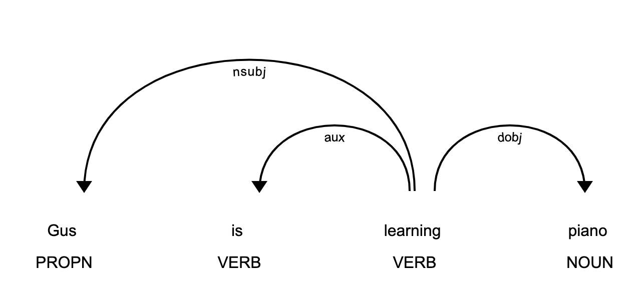
>>> piano_text='Gus is learning piano'>>> piano_doc=nlp(piano_text)>>> fortokeninpiano_doc:... print(token.text,token.tag_,token.head.text,token.dep_)...Gus NNP learning nsubjis VBZ learning auxlearning VBG learning ROOTpiano NN learning dobj

In this example, the sentence contains three relationships:

  1. nsubj is the subject of the word. Its headword is a verb.
  2. aux is an auxiliary word. Its headword is a verb.
  3. dobj is the direct object of the verb. Its headword is a verb.

There is a detailed list of relationships with descriptions. You can use displaCy to visualize the dependency tree:

>>>
>>> displacy.serve(piano_doc,style='dep')

This code will produce a visualization that can be accessed by opening http://127.0.0.1:5000 in your browser:

Displacy: Dependency Parse DemodisplaCy: Dependency Parse Demo

This image shows you that the subject of the sentence is the proper noun Gus and that it has a learn relationship with piano.

The dependency parse tree has all the properties of a tree. This tree contains information about sentence structure and grammar and can be traversed in different ways to extract relationships.

spaCy provides attributes like children, lefts, rights, and subtree to navigate the parse tree:

>>>
>>> one_line_about_text=('Gus Proto is a Python developer'... ' currently working for a London-based Fintech company')>>> one_line_about_doc=nlp(one_line_about_text)>>> # Extract children of `developer`>>> print([token.textfortokeninone_line_about_doc[5].children])['a', 'Python', 'working']>>> # Extract previous neighboring node of `developer`>>> print(one_line_about_doc[5].nbor(-1))Python>>> # Extract next neighboring node of `developer`>>> print(one_line_about_doc[5].nbor())currently>>> # Extract all tokens on the left of `developer`>>> print([token.textfortokeninone_line_about_doc[5].lefts])['a', 'Python']>>> # Extract tokens on the right of `developer`>>> print([token.textfortokeninone_line_about_doc[5].rights])['working']>>> # Print subtree of `developer`>>> print(list(one_line_about_doc[5].subtree))[a, Python, developer, currently, working, for, a, London, -,based, Fintech, company]

You can construct a function that takes a subtree as an argument and returns a string by merging words in it:

>>>
>>> defflatten_tree(tree):... return''.join([token.text_with_wsfortokeninlist(tree)]).strip()...>>> # Print flattened subtree of `developer`>>> print(flatten_tree(one_line_about_doc[5].subtree))a Python developer currently working for a London-based Fintech company

You can use this function to print all the tokens in a subtree.

Shallow Parsing

Shallow parsing, or chunking, is the process of extracting phrases from unstructured text. Chunking groups adjacent tokens into phrases on the basis of their POS tags. There are some standard well-known chunks such as noun phrases, verb phrases, and prepositional phrases.

Noun Phrase Detection

A noun phrase is a phrase that has a noun as its head. It could also include other kinds of words, such as adjectives, ordinals, determiners. Noun phrases are useful for explaining the context of the sentence. They help you infer what is being talked about in the sentence.

spaCy has the property noun_chunks on Doc object. You can use it to extract noun phrases:

>>>
>>> conference_text=('There is a developer conference'... ' happening on 21 July 2019 in London.')>>> conference_doc=nlp(conference_text)>>> # Extract Noun Phrases>>> forchunkinconference_doc.noun_chunks:... print(chunk)...a developer conference21 JulyLondon

By looking at noun phrases, you can get information about your text. For example, a developer conference indicates that the text mentions a conference, while the date 21 July lets you know that conference is scheduled for 21 July. You can figure out whether the conference is in the past or the future. London tells you that the conference is in London.

Verb Phrase Detection

A verb phrase is a syntactic unit composed of at least one verb. This verb can be followed by other chunks, such as noun phrases. Verb phrases are useful for understanding the actions that nouns are involved in.

spaCy has no built-in functionality to extract verb phrases, so you’ll need a library called textacy:

Note:

You can use pip to install textacy:

$ pip install textacy

Now that you have textacy installed, you can use it to extract verb phrases based on grammar rules:

>>>
>>> importtextacy>>> about_talk_text=('The talk will introduce reader about Use'... ' cases of Natural Language Processing in'... ' Fintech')>>> pattern=r'(<VERB>?<ADV>*<VERB>+)'>>> about_talk_doc=textacy.make_spacy_doc(about_talk_text,... lang='en_core_web_sm')>>> verb_phrases=textacy.extract.pos_regex_matches(about_talk_doc,pattern)>>> # Print all Verb Phrase>>> forchunkinverb_phrases:... print(chunk.text)...will introduce>>> # Extract Noun Phrase to explain what nouns are involved>>> forchunkinabout_talk_doc.noun_chunks:... print(chunk)...The talkreaderUse casesNatural Language ProcessingFintech

In this example, the verb phrase introduce indicates that something will be introduced. By looking at noun phrases, you can see that there is a talk that will introduce the reader to use cases of Natural Language Processing or Fintech.

The above code extracts all the verb phrases using a regular expression pattern of POS tags. You can tweak the pattern for verb phrases depending upon your use case.

Note: In the previous example, you could have also done dependency parsing to see what the relationships between the words were.

Named Entity Recognition

Named Entity Recognition (NER) is the process of locating named entities in unstructured text and then classifying them into pre-defined categories, such as person names, organizations, locations, monetary values, percentages, time expressions, and so on.

You can use NER to know more about the meaning of your text. For example, you could use it to populate tags for a set of documents in order to improve the keyword search. You could also use it to categorize customer support tickets into relevant categories.

spaCy has the property ents on Doc objects. You can use it to extract named entities:

>>>
>>> piano_class_text=('Great Piano Academy is situated'... ' in Mayfair or the City of London and has'... ' world-class piano instructors.')>>> piano_class_doc=nlp(piano_class_text)>>> forentinpiano_class_doc.ents:... print(ent.text,ent.start_char,ent.end_char,... ent.label_,spacy.explain(ent.label_))...Great Piano Academy 0 19 ORG Companies, agencies, institutions, etc.Mayfair 35 42 GPE Countries, cities, statesthe City of London 46 64 GPE Countries, cities, states

In the above example, ent is a Span object with various attributes:

  • text gives the Unicode text representation of the entity.
  • start_char denotes the character offset for the start of the entity.
  • end_char denotes the character offset for the end of the entity.
  • label_ gives the label of the entity.

spacy.explain gives descriptive details about an entity label. The spaCy model has a pre-trained list of entity classes. You can use displaCy to visualize these entities:

>>>
>>> displacy.serve(piano_class_doc,style='ent')

If you open http://127.0.0.1:5000 in your browser, then you can see the visualization:

Displacy: Named Entity Recognition DemodisplaCy: Named Entity Recognition Demo

You can use NER to redact people’s names from a text. For example, you might want to do this in order to hide personal information collected in a survey. You can use spaCy to do that:

>>>
>>> survey_text=('Out of 5 people surveyed, James Robert,'... ' Julie Fuller and Benjamin Brooks like'... ' apples. Kelly Cox and Matthew Evans'... ' like oranges.')...>>> defreplace_person_names(token):... iftoken.ent_iob!=0andtoken.ent_type_=='PERSON':... return'[REDACTED] '... returntoken.string...>>> defredact_names(nlp_doc):... forentinnlp_doc.ents:... ent.merge()... tokens=map(replace_person_names,nlp_doc)... return''.join(tokens)...>>> survey_doc=nlp(survey_text)>>> redact_names(survey_doc)'Out of 5 people surveyed, [REDACTED] , [REDACTED] and'' [REDACTED] like apples. [REDACTED] and [REDACTED]'' like oranges.'

In this example, replace_person_names() uses ent_iob. It gives the IOB code of the named entity tag using inside-outside-beginning (IOB) tagging. Here, it can assume a value other than zero, because zero means that no entity tag is set.

Conclusion

spaCy is a powerful and advanced library that is gaining huge popularity for NLP applications due to its speed, ease of use, accuracy, and extensibility. Congratulations! You now know:

  • What the foundational terms and concepts in NLP are
  • How to implement those concepts in spaCy
  • How to customize and extend built-in functionalities in spaCy
  • How to perform basic statistical analysis on a text
  • How to create a pipeline to process unstructured text
  • How to parse a sentence and extract meaningful insights from it

[ Improve Your Python With 🐍 Python Tricks 💌 – Get a short & sweet Python Trick delivered to your inbox every couple of days. >> Click here to learn more and see examples ]

Podcast.__init__: Combining Python And SQL To Build A PyData Warehouse

$
0
0
The ecosystem of tools and libraries in Python for data manipulation and analytics is truly impressive, and continues to grow. There are, however, gaps in their utility that can be filled by the capabilities of a data warehouse. In this episode Robert Hodges discusses how the PyData suite of tools can be paired with a data warehouse for an analytics pipeline that is more robust than either can provide on their own. This is a great introduction to what differentiates a data warehouse from a relational database and ways that you can think differently about running your analytical workloads for larger volumes of data.

Summary

The ecosystem of tools and libraries in Python for data manipulation and analytics is truly impressive, and continues to grow. There are, however, gaps in their utility that can be filled by the capabilities of a data warehouse. In this episode Robert Hodges discusses how the PyData suite of tools can be paired with a data warehouse for an analytics pipeline that is more robust than either can provide on their own. This is a great introduction to what differentiates a data warehouse from a relational database and ways that you can think differently about running your analytical workloads for larger volumes of data.

Announcements

  • Hello and welcome to Podcast.__init__, the podcast about Python and the people who make it great.
  • When you’re ready to launch your next app or want to try a project you hear about on the show, you’ll need somewhere to deploy it, so take a look at our friends over at Linode. With 200 Gbit/s private networking, scalable shared block storage, node balancers, and a 40 Gbit/s public network, all controlled by a brand new API you’ve got everything you need to scale up. And for your tasks that need fast computation, such as training machine learning models, they just launched dedicated CPU instances. Go to pythonpodcast.com/linode to get a $20 credit and launch a new server in under a minute. And don’t forget to thank them for their continued support of this show!
  • Taking a look at recent trends in the data science and analytics landscape, it’s becoming increasingly advantageous to have a deep understanding of both SQL and Python. A hybrid model of analytics can achieve a more harmonious relationship between the two languages. Read more about the Python and SQL Intersection in Analytics at mode.com/init. Specifically, we’re going to be focusing on their similarities, rather than their differences.
  • You listen to this show to learn and stay up to date with the ways that Python is being used, including the latest in machine learning and data analysis. For even more opportunities to meet, listen, and learn from your peers you don’t want to miss out on this year’s conference season. We have partnered with organizations such as O’Reilly Media, Dataversity, Corinium Global Intelligence, and Data Council. Upcoming events include the O’Reilly AI conference, the Strata Data conference, the combined events of the Data Architecture Summit and Graphorum, and Data Council in Barcelona. Go to pythonpodcast.com/conferences to learn more about these and other events, and take advantage of our partner discounts to save money when you register today.
  • Your host as usual is Tobias Macey and today I’m interviewing Robert Hodges about how the PyData ecosystem can play nicely with data warehouses

Interview

  • Introductions
  • How did you get introduced to Python?
  • To start with, can you give a quick overview of what a data warehouse is and how it differs from a "regular" database for anyone who isn’t familiar with them?
    • What are the cases where a data warehouse would be preferable and when are they the wrong choice?
  • What capabilities does a data warehouse add to the PyData ecosystem?
  • For someone who doesn’t yet have a warehouse, what are some of the differentiating factors among the systems that are available?
  • Once you have a data warehouse deployed, how does it get populated and how does Python fit into that workflow?
  • For an analyst or data scientist, how might they interact with the data warehouse and what tools would they use to do so?
  • What are some potential bottlenecks when dealing with the volumes of data that can be contained in a warehouse within Python?
    • What are some ways that you have found to scale beyond those bottlenecks?
  • How does the data warehouse fit into the workflow for a machine learning or artificial intelligence project?
  • What are some of the limitations of data warehouses in the context of the Python ecosystem?
  • What are some of the trends that you see going forward for the integration of the PyData stack with data warehouses?
    • What are some challenges that you anticipate the industry running into in the process?
  • What are some useful references that you would recommend for anyone who wants to dig deeper into this topic?

Keep In Touch

Picks

Closing Announcements

  • Thank you for listening! Don’t forget to check out our other show, the Data Engineering Podcast for the latest on modern data management.
  • Visit the site to subscribe to the show, sign up for the mailing list, and read the show notes.
  • If you’ve learned something or tried out a project from the show then tell us about it! Email hosts@podcastinit.com) with your story.
  • To help other people find the show please leave a review on iTunes and tell your friends and co-workers
  • Join the community in the new Zulip chat workspace at pythonpodcast.com/chat

Links

The intro and outro music is from Requiem for a Fish The Freak Fandango Orchestra / CC BY-SA

PyBites: How to Cleanup S3 Objects and Unittest it

$
0
0

In this guest post Giuseppe shares what he learned having to cleanup a large number of objects in an S3 bucket. He introduces us to some boto3 as well as moto and freezegun he used to test his code. Enter Giuseppe ...

Delete S3 objects

This is a bit of code I wrote for a much bigger script used to monitor and cleanup objects inside an S3 bucket. The rest of the script is proprietary and unfortunately cannot be shared.

The script.py module contains the cleanup() function. It uses boto3 to connect to AWS, pull a list of all the objects contained in a specific bucket and then delete all the ones older than n days.

I have included a few examples of creating a boto3.client which is what the function is expecting as the first argument. The other arguments are used to build the path to the directory inside the S3 bucket where the files are located. This path in AWS terms is called a Prefix.

As the number of the objects in the bucket can be larger than 1000, which is the limit for a single GET in the GET Bucket (List Objects) v2, I used a paginator to pull the entire list. The objects removal follow the same principle and process batches of 1000 objects.

Testing the code

Now this was all good and fun but the really interesting part was how to unittest this code, see test_script.py.

After some researching I found moto, the Mock AWS Services library. It's brilliant! Using this library the test will mock access to the S3 bucket and create several objects in the bucket. You can leave the dummy AWS credentials in the script as they won't be needed.

At this point I wanted to create multiple objects in the S3 mocked environment with different timestamps, but unfortunately I discovered that this was not possible. Once an S3 object is created its creation date (metadata) cannot be easily altered, see the object-metadata docs for reference.

Enter another awesome library called freezegun. I ended up using freeze_time in my tests to mock the date/time and create S3 objects with different timestamps. This way we can safely experiment with the logic of cleanup(), that is leaving objects older than n days and deleting everything else within the prefix.

Here is the test script's output:

$ python test_script.py 
mock-root-prefix/mock-sub-prefix/test_object_01 2019-08-29 00:00:00+00:00
mock-root-prefix/mock-sub-prefix/test_object_02 2019-08-28 00:00:00+00:00
mock-root-prefix/mock-sub-prefix/test_object_03 2019-08-27 00:00:00+00:00
mock-root-prefix/mock-sub-prefix/test_object_04 2019-08-26 00:00:00+00:00
mock-root-prefix/mock-sub-prefix/test_object_05 2019-08-25 00:00:00+00:00
mock-root-prefix/mock-sub-prefix/test_object_06 2019-08-24 00:00:00+00:00
<class 'botocore.client.S3'>
Cleanup S3 backups
Working in the bucket:         my-mock-bucket
The prefix is:                 mock-root-prefix/mock-sub-prefix/
The threshold (n. days) is:    4
Total number of files in the bucket:     7
Number of files to be deleted:           3
Deleting the files from the bucket ...
Deleted:        3
Left to delete: 0
.
----------------------------------------------------------------------
Ran 1test in 0.798s

OK

Again you can find the code for this project here.


Keep Calm and Code in Python!

-- Giuseppe

Codementor: 9 Django Concepts Part 3 - Read Time: 3 Mins

$
0
0
The final part of a 3 part series on 9 concepts of Django to help any aspiring Django developer to accelerate their learnings

Kushal Das: When governments attack: malware campaigns against activists and journalists

$
0
0

Eva

This year at Nullcon Eva gave her talk on When governments attack: malware campaigns against activists and journalists. After introducing EFF, she explained about Dark Caracal, a possibly state-sponsored malware campaign. If we leave aside all technical aspects, this talk has a few other big points to remember.

  • No work is done by a single rock star; this project was a collaboration between people from Lookout and EFF.
  • We should take an ethics class before writing a "Hello World" program in computer science classes.
  • People have the choice of not working for any group who will use your technical skills to abuse human rights

Please watch this talk and tell me over Twitter what do you think.


Kushal Das: stylesheet for nmap output

$
0
0

nmap is the most loved network discovery, and security auditing tool out there. It is already 22 years old and has a ton of features. It can generate output in various formats, including one which is useful for grep, and also one XML output.

We also have one XML stylesheet project for the XML output from nmap.

Click on this result to view the output. You can use this to share the result with someone else, where people can view it from a web-browser with better UI.

The following command was used to generate the output. I already downloaded the stylesheet in the local folder.

nmap -sC -sV -oA toots toots.dgplug.org --stylesheet nmap-bootstrap.xsl

Stack Abuse: Python for NLP: Working with Facebook FastText Library

$
0
0

This is the 20th article in my series of articles on Python for NLP. In the last few articles, we have been exploring deep learning techniques to perform a variety of machine learning tasks, and you should also be familiar with the concept of word embeddings. Word embeddings is a way to convert textual information into numeric form, which in turn can be used as input to statistical algorithms. In my article on word embeddings, I explained how we can create our own word embeddings and how we can use built-in word embeddings such as GloVe.

In this article, we are going to study FastText which is another extremely useful module for word embedding and text classification. FastText has been developed by Facebook and has shown excellent results on many NLP problems, such as semantic similarity detection and text classification.

In this article, we will briefly explore the FastText library. This article is divided into two sections. In the first section, we will see how FastText library creates vector representations that can be used to find semantic similarities between the words. In the second section, we will see the application of FastText library for text classification.

FastText for Semantic Similarity

FastText supports both Continuous Bag of Words and Skip-Gram models. In this article, we will implement the skip-gram model to learn vector representation of words from the Wikipedia articles on artificial intelligence, machine learning, deep learning, and neural networks. Since these topics are quite similar, we chose these topics to have a substantial amount of data to create a corpus. You can add more topics of the similar nature if you want.

As a first step, we need to import the required libraries. We will make use of the Wikipedia library for Python, which can be downloaded via the following command:

$ pip install wikipedia

Importing Libraries

The following script imports the required libraries into our application:

from keras.preprocessing.text import Tokenizer
from gensim.models.fasttext import FastText
import numpy as np
import matplotlib.pyplot as plt
import nltk
from string import punctuation
from nltk.corpus import stopwords
from nltk.tokenize import word_tokenize
from nltk.stem import WordNetLemmatizer
from nltk.tokenize import sent_tokenize
from nltk import WordPunctTokenizer

import wikipedia
import nltk
nltk.download('punkt')
nltk.download('wordnet')
nltk.download('stopwords')
en_stop = set(nltk.corpus.stopwords.words('english'))

%matplotlib inline

You can see that we are using the FastText module from the gensim.models.fasttext library. For the word representation and semantic similarity, we can use the Gensim model for FastText. This model can run on Windows, however, for text classification, we will have to use Linux platform. We will see that in the next section.

Scraping Wikipedia Articles

In this step, we will scrape the required Wikipedia articles. Look at the script below:

artificial_intelligence = wikipedia.page("Artificial Intelligence").content
machine_learning = wikipedia.page("Machine Learning").content
deep_learning = wikipedia.page("Deep Learning").content
neural_network = wikipedia.page("Neural Network").content

artificial_intelligence = sent_tokenize(artificial_intelligence)
machine_learning = sent_tokenize(machine_learning)
deep_learning = sent_tokenize(deep_learning)
neural_network = sent_tokenize(neural_network)

artificial_intelligence.extend(machine_learning)
artificial_intelligence.extend(deep_learning)
artificial_intelligence.extend(neural_network)

To scrape a Wikipedia page, we can use the page method from the wikipedia module. The name of the page that you want to scrap is passed as a parameter to the page method. The method returns WikipediaPage object, which you can then use to retrieve the page contents via the content attribute, as shown in the above script.

The scraped content from the four Wikipedia pages are then tokenized into sentences using the sent_tokenize method. The sent_tokenize method returns list of sentences. The sentences for the four pages are tokenized separately. Finally, sentences from the four articles are joined together via the extend method.

Data Preprocessing

The next step is to clean our text data by removing punctuations and numbers. We will also convert the data into the lower case. The words in our data will be lemmatized to their root form. Furthermore, the stop words and the words with the length less than 4 will be removed from the corpus.

The preprocess_text function, as defined below performs the preprocessing tasks.

import re
from nltk.stem import WordNetLemmatizer

stemmer = WordNetLemmatizer()

def preprocess_text(document):
        # Remove all the special characters
        document = re.sub(r'\W', ' ', str(document))

        # remove all single characters
        document = re.sub(r'\s+[a-zA-Z]\s+', ' ', document)

        # Remove single characters from the start
        document = re.sub(r'\^[a-zA-Z]\s+', ' ', document)

        # Substituting multiple spaces with single space
        document = re.sub(r'\s+', ' ', document, flags=re.I)

        # Removing prefixed 'b'
        document = re.sub(r'^b\s+', '', document)

        # Converting to Lowercase
        document = document.lower()

        # Lemmatization
        tokens = document.split()
        tokens = [stemmer.lemmatize(word) for word in tokens]
        tokens = [word for word in tokens if word not in en_stop]
        tokens = [word for word in tokens if len(word) > 3]

        preprocessed_text = ' '.join(tokens)

        return preprocessed_text

Let's see if our function performs the desired task by preprocessing a dummy sentence:

sent = preprocess_text("Artificial intelligence, is the most advanced technology of the present era")
print(sent)

The preprocessed sentence looks like this:

artificial intelligence advanced technology present

You can see the punctuations and stop words have been removed, and the sentences have been lemmatized. Furthermore, words with length less than 4, such as "era", have also been removed. These choices were chosen randomly for this test, so you may allow the words with smaller or greater lengths in the corpus.

Creating Words Representation

We have preprocessed our corpus. Now is the time to create word representations using FastText. Let's first define the hyper-parameters for our FastText model:

embedding_size = 60
window_size = 40
min_word = 5
down_sampling = 1e-2

Here embedding_size is the size of the embedding vector. In other words, each word in our corpus will be represented as a 60-dimensional vector. The window_size is the size of the number of words occurring before and after the word based on which the word representations will be learned for the word. This might sound tricky, however in the skip-gram model we input a word to the algorithm and the output is the context words. If the window size is 40, for each input there will be 80 outputs: 40 words that occur before the input word and 40 words that occur after the input word. The word embeddings for the input word are learned using these 80 output words.

The next hyper-parameter is the min_word, which specifies the minimum frequency of a word in the corpus for which the word representations will be generated. Finally, the most frequently occurring word will be down-sampled by a number specified by the down_sampling attribute.

Let's now create our FastText model for word representations.

%%time
ft_model = FastText(word_tokenized_corpus,
                      size=embedding_size,
                      window=window_size,
                      min_count=min_word,
                      sample=down_sampling,
                      sg=1,
                      iter=100)

All the parameters in the above script are self-explanatory, except sg. The sg parameter defines the type of model that we want to create. A value of 1 specifies that we want to create skip-gram model. Whereas zero specifies the bag of words model, which is the default value as well.

Execute the above script. It may take some time to run. On my machine the time statistics for the above code to run are as follows:

CPU times: user 1min 45s, sys: 434 ms, total: 1min 45s
Wall time: 57.2 s

Let's now see the word representation for the word "artificial". To do so, you can use the wv method of the FastText object and pass it the name of the word inside a list.

print(ft_model.wv['artificial'])

Here is the output:

[-3.7653010e-02 -4.5558015e-01  3.2035065e-01 -1.5289043e-01
  4.0645871e-02 -1.8946664e-01  7.0426887e-01  2.8806925e-01
 -1.8166199e-01  1.7566417e-01  1.1522485e-01 -3.6525184e-01
 -6.4378887e-01 -1.6650060e-01  7.4625671e-01 -4.8166099e-01
  2.0884991e-01  1.8067230e-01 -6.2647951e-01  2.7614883e-01
 -3.6478557e-02  1.4782918e-02 -3.3124462e-01  1.9372456e-01
  4.3028224e-02 -8.2326338e-02  1.0356739e-01  4.0792203e-01
 -2.0596240e-02 -3.5974573e-02  9.9928051e-02  1.7191900e-01
 -2.1196717e-01  6.4424530e-02 -4.4705093e-02  9.7391091e-02
 -2.8846195e-01  8.8607501e-03  1.6520244e-01 -3.6626378e-01
 -6.2017748e-04 -1.5083785e-01 -1.7499258e-01  7.1994811e-02
 -1.9868813e-01 -3.1733567e-01  1.9832127e-01  1.2799081e-01
 -7.6522082e-01  5.2335665e-02 -4.5766738e-01 -2.7947658e-01
  3.7890410e-03 -3.8761377e-01 -9.3001537e-02 -1.7128626e-01
 -1.2923178e-01  3.9627206e-01 -3.6673656e-01  2.2755004e-01]

In the output above, you can see a 60-dimensional vector for the word "artificial"

Let's now find top 5 most similar words for the words 'artificial', 'intelligence', 'machine', 'network', 'recurrent', 'deep'. You can chose any number of words. The following script prints the specified words along with the 5 most similar words.

semantically_similar_words = {words: [item[0] for item in ft_model.wv.most_similar([words], topn=5)]
                  for words in ['artificial', 'intelligence', 'machine', 'network', 'recurrent', 'deep']}

for k,v in semantically_similar_words.items():
    print(k+":"+str(v))

The output is as follows:

artificial:['intelligence', 'inspired', 'book', 'academic', 'biological']
intelligence:['artificial', 'human', 'people', 'intelligent', 'general']
machine:['ethic', 'learning', 'concerned', 'argument', 'intelligence']
network:['neural', 'forward', 'deep', 'backpropagation', 'hidden']
recurrent:['rnns', 'short', 'schmidhuber', 'shown', 'feedforward']
deep:['convolutional', 'speech', 'network', 'generative', 'neural']

We can also find the cosine similarity between the vectors for any two words, as shown below:

print(ft_model.wv.similarity(w1='artificial', w2='intelligence'))

The output shows a value of "0.7481". The value can be anywhere between 0 and 1. A higher value means higher similarity.

Visualizing Word Similarities

Though each word in our model is represented as 60-dimensional vector, we can use principal component analysis technique to find two principal components. The two principal components can then be used to plot the words in a two dimensional space. However, first we need to create a list of all the words in the semantically_similar_words dictionary. The following script does that:

from sklearn.decomposition import PCA

all_similar_words = sum([[k] + v for k, v in semantically_similar_words.items()], [])

print(all_similar_words)
print(type(all_similar_words))
print(len(all_similar_words))

In the script above, we iterate through all the key-value pairs in the semantically_similar_words dictionary. Each key in the dictionary is a word. The corresponding value is a list of all semantically similar words. Since we found the top 5 most similar words for a list of 6 words i.e. 'artificial', 'intelligence', 'machine', 'network', 'recurrent', 'deep', you will see that there will be 30 items in the all_similar_words list.

Next, we have to find the word vectors for all these 30 words, and then use PCA to reduce the dimensions of the word vectors from 60 to 2. We can then use the plt method, which is an alias of the matplotlib.pyplot method to plot the words on a two-dimensional vector space.

Execute the following script to visualize the words:

word_vectors = ft_model.wv[all_similar_words]

pca = PCA(n_components=2)

p_comps = pca.fit_transform(word_vectors)
word_names = all_similar_words

plt.figure(figsize=(18, 10))
plt.scatter(p_comps[:, 0], p_comps[:, 1], c='red')

for word_names, x, y in zip(word_names, p_comps[:, 0], p_comps[:, 1]):
    plt.annotate(word_names, xy=(x+0.06, y+0.03), xytext=(0, 0), textcoords='offset points')

The output of the above script looks like this:

alt

You can see the words that frequently occur together in the text are close to each other in the two dimensional plane as well. For instance, the words "deep" and "network" are almost overlapping. Similarly, the words "feedforward" and "backpropagation" are also very close.

Now we know how to create word embeddings using FastText. In the next section, we will see how FastText can be used for text classification tasks.

FastText for Text Classification

Text classification refers to classifying textual data into predefined categories based on the contents of the text. Sentiment analysis, spam detection, and tag detection are some of the most common examples of use-cases for text classification.

FastText text classification module can only be run via Linux or OSX. If you are a Windows user, you can use Google Colaboratory to run FastText text classification module. All the scripts in this section have been run using Google Colaboratory.

The Dataset

The dataset for this article can be downloaded from this Kaggle link. The dataset contains multiple files, but we are only interested in the yelp_review.csv file. The file contains more than 5.2 million reviews about different businesses including restaurants, bars, dentists, doctors, beauty salons, etc. However, we will only be using the first 50,000 records to train our model due to memory constraints. You can try with more records if you want.

Let's import the required libraries and load the dataset:

import pandas as pd
import numpy as np

yelp_reviews = pd.read_csv("/content/drive/My Drive/Colab Datasets/yelp_review_short.csv")

bins = [0,2,5]
review_names = ['negative', 'positive']

yelp_reviews['reviews_score'] = pd.cut(yelp_reviews['stars'], bins, labels=review_names)

yelp_reviews.head()

In the script above we load the yelp_review_short.csv file that contains 50,000 reviews with the pd.read_csv function.

We will simplify our problem by converting the numerical values for the reviews into categorical ones. This will be done by adding a new column ,reviews_score, to our dataset. If the user review has a value between 1-2 in the Stars column (which rates the business on a 1-5 scale), the reviews_score column will have a string value negative. If the rating is between 3-5 in the Stars column, the reviews_score column will contain a value positive. This makes our problem, a binary classification problem.

Finally the header of the dataframe is printed as shown below:

alt

Installing FastText

The next step is to import FastText models, which can be imported using the wget command from the GitHub repository, as shown in the following script:

!wget https://github.com/facebookresearch/fastText/archive/v0.1.0.zip

Note: If you are executing the above command from a Linux terminal, you don't have to prefix ! before the above command. In Google Colaboratory notebook, any command after the ! is executed as a shell command and not within the Python interpreter. Hence all non-Python commands here are prefixed by !.

If you run the above script and see the following results, that means FastText has been successfully downloaded:

--2019-08-16 15:05:05--  https://github.com/facebookresearch/fastText/archive/v0.1.0.zip
Resolving github.com (github.com)... 140.82.113.4
Connecting to github.com (github.com)|140.82.113.4|:443... connected.
HTTP request sent, awaiting response... 302 Found
Location: https://codeload.github.com/facebookresearch/fastText/zip/v0.1.0 [following]
--2019-08-16 15:05:05--  https://codeload.github.com/facebookresearch/fastText/zip/v0.1.0
Resolving codeload.github.com (codeload.github.com)... 192.30.255.121
Connecting to codeload.github.com (codeload.github.com)|192.30.255.121|:443... connected.
HTTP request sent, awaiting response... 200 OK
Length: unspecified [application/zip]
Saving to: ‘v0.1.0.zip’

v0.1.0.zip              [ <=>                ]  92.06K  --.-KB/s    in 0.03s

2019-08-16 15:05:05 (3.26 MB/s) - ‘v0.1.0.zip’ saved [94267]

The next step is to unzip FastText modules. Simply type the following command:

!unzip v0.1.0.zip

Next, you have to navigate to the directory where you downloaded FastText and then execute the !make command to run C++ binaries. Execute the following steps:

cd fastText-0.1.0
!make

If you see the following output, that means FastText is successfully installed on your machine.

c++ -pthread -std=c++0x -O3 -funroll-loops -c src/args.cc
c++ -pthread -std=c++0x -O3 -funroll-loops -c src/dictionary.cc
c++ -pthread -std=c++0x -O3 -funroll-loops -c src/productquantizer.cc
c++ -pthread -std=c++0x -O3 -funroll-loops -c src/matrix.cc
c++ -pthread -std=c++0x -O3 -funroll-loops -c src/qmatrix.cc
c++ -pthread -std=c++0x -O3 -funroll-loops -c src/vector.cc
c++ -pthread -std=c++0x -O3 -funroll-loops -c src/model.cc
c++ -pthread -std=c++0x -O3 -funroll-loops -c src/utils.cc
c++ -pthread -std=c++0x -O3 -funroll-loops -c src/fasttext.cc
c++ -pthread -std=c++0x -O3 -funroll-loops args.o dictionary.o productquantizer.o matrix.o qmatrix.o vector.o model.o utils.o fasttext.o src/main.cc -o fasttext

To verify the installation, execute the following command:

!./fasttext

You should see that these commands are supported by FastText:

usage: fasttext <command> <args>

The commands supported by FastText are:

  supervised              train a supervised classifier
  quantize                quantize a model to reduce the memory usage
  test                    evaluate a supervised classifier
  predict                 predict most likely labels
  predict-prob            predict most likely labels with probabilities
  skipgram                train a skipgram model
  cbow                    train a cbow model
  print-word-vectors      print word vectors given a trained model
  print-sentence-vectors  print sentence vectors given a trained model
  nn                      query for nearest neighbors
  analogies               query for analogies

Text Classification

Before we train FastText models to perform text classification, it is pertinent to mention that FastText accepts data in a special format, which is as follows:

_label_tag This is sentence 1
_label_tag2 This is sentence 2.

If we look at our dataset, it is not in the desired format. The text with positive sentiment should look like this:

__label__positive burgers are very big portions here.

Similarly, negative reviews should look like this:

__label__negative They do not use organic ingredients, but I thi...

The following script filters the reviews_score and text columns from the dataset and then prefixes __label__ before all the values in the reviews_score column. Similarly, the \n and \t are replaced by a space in the text column. Finally, the updated dataframe is written to the disk in the form of yelp_reviews_updated.txt.

import pandas as pd
from io import StringIO
import csv

col = ['reviews_score', 'text']

yelp_reviews = yelp_reviews[col]
yelp_reviews['reviews_score']=['__label__'+ s for s in yelp_reviews['reviews_score']]
yelp_reviews['text']= yelp_reviews['text'].replace('\n',' ', regex=True).replace('\t',' ', regex=True)
yelp_reviews.to_csv(r'/content/drive/My Drive/Colab Datasets/yelp_reviews_updated.txt', index=False, sep=' ', header=False, quoting=csv.QUOTE_NONE, quotechar="", escapechar=" ")

Let's now print the head of the updated yelp_reviews dataframe.

yelp_reviews.head()

You should see the following results:

reviews_score   text
0   __label__positive   Super simple place but amazing nonetheless. It...
1   __label__positive   Small unassuming place that changes their menu...
2   __label__positive   Lester's is located in a beautiful neighborhoo...
3   __label__positive   Love coming here. Yes the place always needs t...
4   __label__positive   Had their chocolate almond croissant and it wa...

Similarly, the tail of the dataframe looks like this:

    reviews_score   text
49995   __label__positive   This is an awesome consignment store! They hav...
49996   __label__positive   Awesome laid back atmosphere with made-to-orde...
49997   __label__positive   Today was my first appointment and I can hones...
49998   __label__positive   I love this chic salon. They use the best prod...
49999   __label__positive   This place is delicious. All their meats and s...

We have converted our dataset into the required shape. The next step is to divide our data into train and test sets. The 80% data i.e. the first 40,000 records out of 50,000 records will be used to train the data, while 20% data (the last 10,000 records) will be used to evaluate the performance of the algorithm.

The following script divides the data into training and test sets:

!head -n 40000 "/content/drive/My Drive/Colab Datasets/yelp_reviews_updated.txt" > "/content/drive/My Drive/Colab Datasets/yelp_reviews_train.txt"
!tail -n 10000 "/content/drive/My Drive/Colab Datasets/yelp_reviews_updated.txt" > "/content/drive/My Drive/Colab Datasets/yelp_reviews_test.txt"

Once the above script is executed, the yelp_reviews_train.txt file will be generated, which contains the training data. Similarly, the newly generated yelp_reviews_test.txt file will contain test data.

Now is the time to train our FastText text classification algorithm.

%%time
!./fasttext supervised -input "/content/drive/My Drive/Colab Datasets/yelp_reviews_train.txt" -output model_yelp_reviews

To train the algorithm we have to use supervised command and pass it the input file. The model name is specified after the -output keyword. The above script will result in a trained text classification model called model_yelp_reviews.bin. Here is the output for the script above:

Read 4M words
Number of words:  177864
Number of labels: 2
Progress: 100.0%  words/sec/thread: 2548017  lr: 0.000000  loss: 0.246120  eta: 0h0m
CPU times: user 212 ms, sys: 48.6 ms, total: 261 ms
Wall time: 15.6 s

You can take a look at the model via !ls command as shown below:

!ls

Here is the output:

args.o             Makefile         quantization-results.sh
classification-example.sh  matrix.o         README.md
classification-results.sh  model.o          src
CONTRIBUTING.md        model_yelp_reviews.bin   tutorials
dictionary.o           model_yelp_reviews.vec   utils.o
eval.py            PATENTS          vector.o
fasttext           pretrained-vectors.md    wikifil.pl
fasttext.o         productquantizer.o       word-vector-example.sh
get-wikimedia.sh       qmatrix.o            yelp_reviews_train.txt
LICENSE            quantization-example.sh

You can see the model_yelp_reviews.bin in the above list of documents.

Finally, to test the model you can use the test command. You have to specify the model name and the test file after the test command, as shown below:

!./fasttext test model_yelp_reviews.bin "/content/drive/My Drive/Colab Datasets/yelp_reviews_test.txt"

The output of the above script looks like this:

N   10000
P@1 0.909
R@1 0.909
Number of examples: 10000

Here P@1 refers to precision and R@1refers to recall. You can see our model achieves precision and recall of 0.909 which is pretty good.

Let's now try to clean our text of punctuations, special characters, and convert it into the lower case to improve the uniformity of text. The following script cleans the train set:

!cat "/content/drive/My Drive/Colab Datasets/yelp_reviews_train.txt" | sed -e "s/\([.\!?,’/()]\)/ \1 /g" | tr "[:upper:]" "[:lower:]" > "/content/drive/My Drive/Colab Datasets/yelp_reviews_train_clean.txt"

And the following script cleans the test set:

"/content/drive/My Drive/Colab Datasets/yelp_reviews_test.txt" | sed -e "s/\([.\!?,’/()]\)/ \1 /g" | tr "[:upper:]" "[:lower:]" > "/content/drive/My Drive/Colab Datasets/yelp_reviews_test_clean.txt"

Now, we will train the model on the cleaned training set:

%%time
!./fasttext supervised -input "/content/drive/My Drive/Colab Datasets/yelp_reviews_train_clean.txt" -output model_yelp_reviews

And finally, we will use the model trained on cleaned training set to make predictions on the cleaned test set:

!./fasttext test model_yelp_reviews.bin "/content/drive/My Drive/Colab Datasets/yelp_reviews_test_clean.txt"

The output of the above script is as follows:

N   10000
P@1 0.915
R@1 0.915
Number of examples: 10000

You can see a slight increase in both precision and recall. To further improve the model, you can increase the epochs and learning rate of the model. The following script sets the number of epochs to 30 and learning rate to 0.5.

%%time
!./fasttext supervised -input "/content/drive/My Drive/Colab Datasets/yelp_reviews_train_clean.txt" -output model_yelp_reviews -epoch 30 -lr 0.5

You can try different numbers and see if you can get better results. Don't forget to share your results in the comments!

Conclusion

FastText model has recently been proved state of the art for word embeddings and text classification tasks on many datasets. It is very easy to use and lightning fast as compared to other word embedding models.

In this article, we briefly explored how to find semantic similarities between different words by creating word embeddings using FastText. The second part of the article explains how to perform text classification via FastText library.

PyCharm: Webinar: “10 Tools and Techniques Python Web Developers Should Explore” with Michael Kennedy

$
0
0

Building web applications is one of Python’s true superpowers. Yet, the wide-open ecosystem means there are SO MANY CHOICES for any given project. How do you know whether you’re using the right tool for the right problem?

  • Wednesday, September 25th
  • 6:00 PM – 7:00 PM CEST (12:00 PM – 1:00 PM EDT)
  • Register here
  • Aimed at intermediate Python developers

webinar2019_watch the recording-17

In this webcast, you will go on a tour of modern Python-based web techniques and tooling. We’ll see how to get the most out of your web app’s scalability with async and await. Host multi-container applications in Docker Compose. Leverage the popular and powerful JavaScript front-end frameworks when it makes sense. We’ll cover these and much more during the webcast.

Speaking To You

Michael Kennedy is the host of Talk Python to Me and co-host of Python Bytes podcasts. He is also the founder of Talk Python training and a Python Software Foundation fellow. Michael has a PyCharm course and is co-author of the book Effective PyCharm. Michael has been working in the developer field for more than 20 years and has spoken at numerous conferences.

ListenData: Pandas Tutorial : Step by Step Guide (50 Examples)

$
0
0
Pandas being one of the most popular package in Python is widely used for data manipulation. It is a very powerful and versatile package which makes data cleaning and wrangling much easier and pleasant.
The Pandas library has a great contribution to the python community and it makes python as one of the top programming language for data science and analytics. It has become first choice of data analysts and scientists for data analysis and manipulation.

pandas tutorial
Data Analysis with Python : Pandas Step by Step Guide

Why to use pandas package?
It has many functions which are the essence for data handling and manipulation. In short, it can perform the following tasks for you -
  1. Create a structured data set similar to R's data frame and Excel spreadsheet.
  2. Reading data from various sources such as CSV, TXT, XLSX, SQL database, R etc.
  3. Selecting particular rows or columns from data set
  4. Arranging data in ascending or descending order
  5. Filtering data based on some conditions
  6. Summarizing data by classification variable
  7. Reshape data into wide or long format
  8. Time series analysis
  9. Merging and concatenating two datasets
  10. Iterate over the rows of dataset
  11. Writing or Exporting data in CSV or Excel format

Datasets:
In this tutorial we will use two datasets: 'income' and 'iris'.
  1. 'income' data : This data contains the income of various states from 2002 to 2015. The dataset contains 51 observations and 16 variables. Download link
  2. 'iris' data: It comprises of 150 observations with 5 variables. We have 3 species of flowers(50 flowers for each specie) and for all of them the sepal length and width and petal length and width are given. Download link 


Important pandas functions to remember
The following is a list of common tasks along with pandas functions.
UtilityFunctions
Extract Column Namesdf.columns
Select first 2 rowsdf.iloc[:2]
Select first 2 columnsdf.iloc[:,:2]
Select columns by namedf.loc[:,["col1","col2"]]
Select random no. of rowsdf.sample(n = 10)
Select fraction of random rowsdf.sample(frac = 0.2)
Rename the variablesdf.rename( )
Selecting a column as indexdf.set_index( )
Removing rows or columnsdf.drop( )
Sorting valuesdf.sort_values( )
Grouping variablesdf.groupby( )
Filteringdf.query( )
Finding the missing valuesdf.isnull( )
Dropping the missing valuesdf.dropna( )
Removing the duplicatesdf.drop_duplicates( )
Creating dummiespd.get_dummies( )
Rankingdf.rank( )
Cumulative sumdf.cumsum( )
Quantilesdf.quantile( )
Selecting numeric variablesdf.select_dtypes( )
Concatenating two dataframespd.concat()
Merging on basis of common variablepd.merge( )
Importing pandas library
You need to import or load the Pandas library first in order to use it. By "Importing a library", it means loading it into the memory and then you can use it. Run the following code to import pandas library:
import pandas as pd
The "pd" is an alias or abbreviation which will be used as a shortcut to access or call pandas functions. To access the functions from pandas library, you just need to type pd.function instead of  pandas.function every time you need to apply it.

Importing Dataset
To read or import data from CSV file, you can use read_csv() function. In the function, you need to specify the file location of your CSV file.
income = pd.read_csv("C:\\Users\\Hp\\Python\\Basics\\income.csv")
 Index       State    Y2002    Y2003    Y2004    Y2005    Y2006    Y2007  \
0 A Alabama 1296530 1317711 1118631 1492583 1107408 1440134
1 A Alaska 1170302 1960378 1818085 1447852 1861639 1465841
2 A Arizona 1742027 1968140 1377583 1782199 1102568 1109382
3 A Arkansas 1485531 1994927 1119299 1947979 1669191 1801213
4 C California 1685349 1675807 1889570 1480280 1735069 1812546

Y2008 Y2009 Y2010 Y2011 Y2012 Y2013 Y2014 Y2015
0 1945229 1944173 1237582 1440756 1186741 1852841 1558906 1916661
1 1551826 1436541 1629616 1230866 1512804 1985302 1580394 1979143
2 1752886 1554330 1300521 1130709 1907284 1363279 1525866 1647724
3 1188104 1628980 1669295 1928238 1216675 1591896 1360959 1329341
4 1487315 1663809 1624509 1639670 1921845 1156536 1388461 1644607

Get Variable Names
By using income.columnscommand, you can fetch the names of variables of a data frame.
Index(['Index', 'State', 'Y2002', 'Y2003', 'Y2004', 'Y2005', 'Y2006', 'Y2007',
'Y2008', 'Y2009', 'Y2010', 'Y2011', 'Y2012', 'Y2013', 'Y2014', 'Y2015'],
dtype='object')
income.columns[0:2] returns first two column names 'Index', 'State'. In python, indexing starts from 0.

Knowing the Variable types
You can use the dataFrameName.dtypes command to extract the information of types of variables stored in the data frame.
income.dtypes 
Index    object
State object
Y2002 int64
Y2003 int64
Y2004 int64
Y2005 int64
Y2006 int64
Y2007 int64
Y2008 int64
Y2009 int64
Y2010 int64
Y2011 int64
Y2012 int64
Y2013 int64
Y2014 int64
Y2015 int64
dtype: object

Here 'object' means strings or character variables. 'int64' refers to numeric variables (without decimals).

To see the variable type of one variable (let's say "State") instead of all the variables, you can use the command below -
income['State'].dtypes
It returns dtype('O'). In this case, 'O' refers to object i.e. type of variable as character.

Changing the data types
Y2008 is an integer. Suppose we want to convert it to float (numeric variable with decimals) we can write:
income.Y2008 = income.Y2008.astype(float)
income.dtypes
Index     object
State object
Y2002 int64
Y2003 int64
Y2004 int64
Y2005 int64
Y2006 int64
Y2007 int64
Y2008 float64
Y2009 int64
Y2010 int64
Y2011 int64
Y2012 int64
Y2013 int64
Y2014 int64
Y2015 int64
dtype: object

To view the dimensions or shape of the data
income.shape
 (51, 16)

51 is the number of rows and 16 is the number of columns.

You can also use shape[0] to see the number of rows (similar to nrow() in R) and shape[1] for number of columns (similar to ncol() in R). 
income.shape[0]
income.shape[1]

To view only some of the rows
By default head( ) shows first 5 rows. If we want to see a specific number of rows we can mention it in the parenthesis. Similarly tail( ) function shows last 5 rows by default.
income.head()
income.head(2) #shows first 2 rows.
income.tail()
income.tail(2) #shows last 2 rows

Alternatively, any of the following commands can be used to fetch first five rows.
income[0:5]
income.iloc[0:5]

Define Categorical Variable
Like factors() function in R, we can include categorical variable in python using "category" dtype.
s = pd.Series([1,2,3,1,2], dtype="category")
s
0    1
1 2
2 3
3 1
4 2
dtype: category
Categories (3, int64): [1, 2, 3]

Extract Unique Values
The unique() function shows the unique levels or categories in the dataset.
income.Index.unique()
array(['A', 'C', 'D', ..., 'U', 'V', 'W'], dtype=object)


The nunique( ) shows the number of unique values.
income.Index.nunique()
It returns 19 as index column contains distinct 19 values.

Generate Cross Tab
pd.crosstab( ) is used to create a bivariate frequency distribution. Here the bivariate frequency distribution is between Index and State columns.
pd.crosstab(income.Index,income.State)

Creating a frequency distribution
income.Index selects the 'Index' column of 'income' dataset and value_counts( ) creates a frequency distribution. By default ascending = False i.e. it will show the 'Index' having the maximum frequency on the top.
income.Index.value_counts(ascending = True)
F    1
G 1
U 1
L 1
H 1
P 1
R 1
D 2
T 2
S 2
V 2
K 2
O 3
C 3
I 4
W 4
A 4
M 8
N 8
Name: Index, dtype: int64

To draw the samples
income.sample( ) is used to draw random samples from the dataset containing all the columns. Here n = 5 depicts we need 5 columns and frac = 0.1 tells that we need 10 percent of the data as my sample.
income.sample(n = 5)
income.sample(frac = 0.1)
Selecting only a few of the columns
There are multiple ways you can select a particular column. Both the following line of code selects State variable from income data frame.
income["State"]
income.State
To select multiple columns by name, you can use the following syntax.
income[["Index","State","Y2008"]]
To select only specific columns and rows, we use either loc[ ] or iloc[ ] functions. The index or columns to be selected are passed as lists. "Index":"Y2008" denotes the that all the columns from Index to Y2008 are to be selected.
Syntax of df.loc[  ]
df.loc[row_index , column_index]
income.loc[:,["Index","State","Y2008"]]
income.loc[0:2,["Index","State","Y2008"]]  #Selecting rows with Index label 0 to 2 & columns
income.loc[:,"Index":"Y2008"]  #Selecting consecutive columns
#In the above command both Index and Y2008 are included.
income.iloc[:,0:5]  #Columns from 1 to 5 are included. 6th column not included
Difference between loc and iloc
loc considers rows (or columns) with particular labels from the index. Whereas iloc considers rows (or columns) at particular positions in the index so it only takes integers.
x = pd.DataFrame({"var1" : np.arange(1,20,2)}, index=[9,8,7,6,10, 1, 2, 3, 4, 5])
    var1
9 1
8 3
7 5
6 7
10 9
1 11
2 13
3 15
4 17
5 19
iloc Code
x.iloc[:3]

Output:
var1
9 1
8 3
7 5
loc code
x.loc[:3]

Output:
var1
9 1
8 3
7 5
6 7
10 9
1 11
2 13
3 15
Renaming the variables
We create a dataframe 'data' for information of people and their respective zodiac signs.
data = pd.DataFrame({"A" : ["John","Mary","Julia","Kenny","Henry"], "B" : ["Libra","Capricorn","Aries","Scorpio","Aquarius"]})
data 
       A          B
0 John Libra
1 Mary Capricorn
2 Julia Aries
3 Kenny Scorpio
4 Henry Aquarius
If all the columns are to be renamed then we can use data.columns and assign the list of new column names.
#Renaming all the variables.
data.columns = ['Names','Zodiac Signs']

   Names Zodiac Signs
0 John Libra
1 Mary Capricorn
2 Julia Aries
3 Kenny Scorpio
4 Henry Aquarius
If only some of the variables are to be renamed then we can use rename( ) function where the new names are passed in the form of a dictionary.
#Renaming only some of the variables.
data.rename(columns = {"Names":"Cust_Name"},inplace = True)
  Cust_Name Zodiac Signs
0 John Libra
1 Mary Capricorn
2 Julia Aries
3 Kenny Scorpio
4 Henry Aquarius
By default in pandas inplace = False which means that no changes are made in the original dataset. Thus if we wish to alter the original dataset we need to define inplace = True.
Suppose we want to replace only a particular character in the list of the column names then we can use str.replace( ) function. For example, renaming the variables which contain "Y" as "Year"
income.columns = income.columns.str.replace('Y' , 'Year ')
income.columns
Index(['Index', 'State', 'Year 2002', 'Year 2003', 'Year 2004', 'Year 2005',
'Year 2006', 'Year 2007', 'Year 2008', 'Year 2009', 'Year 2010',
'Year 2011', 'Year 2012', 'Year 2013', 'Year 2014', 'Year 2015'],
dtype='object')
Setting one column in the data frame as the index
Using set_index("column name") we can set the indices as that column and that column gets removed.
income.set_index("Index",inplace = True)
income.head()
#Note that the indices have changed and Index column is now no more a column
income.columns
income.reset_index(inplace = True)
income.head()
reset_index( ) tells us that one should use the by default indices.
Removing columns and rows
To drop a column we use drop( ) where the first argument is a list of columns to be removed.

By default axis = 0 which means the operation should take place horizontally, row wise. To remove a column we need to set axis = 1.
income.drop('Index',axis = 1)

#Alternatively
income.drop("Index",axis = "columns")
income.drop(['Index','State'],axis = 1)
income.drop(0,axis = 0)
income.drop(0,axis = "index")
income.drop([0,1,2,3],axis = 0)
 Also inplace = False by default thus no alterations are made in the original dataset.  axis = "columns"  and axis = "index" means the column and row(index) should be removed respectively.
Sorting Data
To sort the data sort_values( ) function is deployed. By default inplace = False and ascending = True.
income.sort_values("State",ascending = False)
income.sort_values("State",ascending = False,inplace = True)
income.Y2006.sort_values() 
We have got duplicated for Index thus we need to sort the dataframe firstly by Index and then for each particular index we sort the values by Y2002
income.sort_values(["Index","Y2002"]) 

Create new variables
Using eval( ) arithmetic operations on various columns can be carried out in a dataset.
income["difference"] = income.Y2008-income.Y2009

#Alternatively
income["difference2"] = income.eval("Y2008 - Y2009")
income.head()
  Index       State    Y2002    Y2003    Y2004    Y2005    Y2006    Y2007  \
0 A Alabama 1296530 1317711 1118631 1492583 1107408 1440134
1 A Alaska 1170302 1960378 1818085 1447852 1861639 1465841
2 A Arizona 1742027 1968140 1377583 1782199 1102568 1109382
3 A Arkansas 1485531 1994927 1119299 1947979 1669191 1801213
4 C California 1685349 1675807 1889570 1480280 1735069 1812546

Y2008 Y2009 Y2010 Y2011 Y2012 Y2013 Y2014 Y2015 \
0 1945229.0 1944173 1237582 1440756 1186741 1852841 1558906 1916661
1 1551826.0 1436541 1629616 1230866 1512804 1985302 1580394 1979143
2 1752886.0 1554330 1300521 1130709 1907284 1363279 1525866 1647724
3 1188104.0 1628980 1669295 1928238 1216675 1591896 1360959 1329341
4 1487315.0 1663809 1624509 1639670 1921845 1156536 1388461 1644607

difference difference2
0 1056.0 1056.0
1 115285.0 115285.0
2 198556.0 198556.0
3 -440876.0 -440876.0
4 -176494.0 -176494.0

income.ratio = income.Y2008/income.Y2009
The above command does not work, thus to create new columns we need to use square brackets.
We can also use assign( ) function but this command does not make changes in the original data as there is no inplace parameter. Hence we need to save it in a new dataset.
data = income.assign(ratio = (income.Y2008 / income.Y2009))
data.head()

Finding Descriptive Statistics
describe( ) is used to find some statistics like mean,minimum, quartiles etc. for numeric variables.
income.describe() #for numeric variables
              Y2002         Y2003         Y2004         Y2005         Y2006  \
count 5.100000e+01 5.100000e+01 5.100000e+01 5.100000e+01 5.100000e+01
mean 1.566034e+06 1.509193e+06 1.540555e+06 1.522064e+06 1.530969e+06
std 2.464425e+05 2.641092e+05 2.813872e+05 2.671748e+05 2.505603e+05
min 1.111437e+06 1.110625e+06 1.118631e+06 1.122030e+06 1.102568e+06
25% 1.374180e+06 1.292390e+06 1.268292e+06 1.267340e+06 1.337236e+06
50% 1.584734e+06 1.485909e+06 1.522230e+06 1.480280e+06 1.531641e+06
75% 1.776054e+06 1.686698e+06 1.808109e+06 1.778170e+06 1.732259e+06
max 1.983285e+06 1.994927e+06 1.979395e+06 1.990062e+06 1.985692e+06

Y2007 Y2008 Y2009 Y2010 Y2011 \
count 5.100000e+01 5.100000e+01 5.100000e+01 5.100000e+01 5.100000e+01
mean 1.553219e+06 1.538398e+06 1.658519e+06 1.504108e+06 1.574968e+06
std 2.539575e+05 2.958132e+05 2.361854e+05 2.400771e+05 2.657216e+05
min 1.109382e+06 1.112765e+06 1.116168e+06 1.103794e+06 1.116203e+06
25% 1.322419e+06 1.254244e+06 1.553958e+06 1.328439e+06 1.371730e+06
50% 1.563062e+06 1.545621e+06 1.658551e+06 1.498662e+06 1.575533e+06
75% 1.780589e+06 1.779538e+06 1.857746e+06 1.639186e+06 1.807766e+06
max 1.983568e+06 1.990431e+06 1.993136e+06 1.999102e+06 1.992996e+06

Y2012 Y2013 Y2014 Y2015
count 5.100000e+01 5.100000e+01 5.100000e+01 5.100000e+01
mean 1.591135e+06 1.530078e+06 1.583360e+06 1.588297e+06
std 2.837675e+05 2.827299e+05 2.601554e+05 2.743807e+05
min 1.108281e+06 1.100990e+06 1.110394e+06 1.110655e+06
25% 1.360654e+06 1.285738e+06 1.385703e+06 1.372523e+06
50% 1.643855e+06 1.531212e+06 1.580394e+06 1.627508e+06
75% 1.866322e+06 1.725377e+06 1.791594e+06 1.848316e+06
max 1.988270e+06 1.994022e+06 1.990412e+06 1.996005e+06
For character or string variables, you can write include = ['object']. It will return total count, maximum occurring string and its frequency
income.describe(include = ['object'])  #Only for strings / objects
To find out specific descriptive statistics of each column of data frame
income.mean()
income.median()
income.agg(["mean","median"])

agg( ) performs aggregation with summary functions like sum, mean, median, min, max etc.

How to run functions for a particular column(s)?
income.Y2008.mean()
income.Y2008.median()
income.Y2008.min()
income.loc[:,["Y2002","Y2008"]].max()

GroupBy function
To group the data by a categorical variable we use groupby( ) function and hence we can do the operations on each category.
income.groupby("Index")["Y2002","Y2003"].min()
        Y2002    Y2003
Index
A 1170302 1317711
C 1343824 1232844
D 1111437 1268673
F 1964626 1468852
G 1929009 1541565
H 1461570 1200280
I 1353210 1438538
K 1509054 1290700
L 1584734 1110625
M 1221316 1149931
N 1395149 1114500
O 1173918 1334639
P 1320191 1446723
R 1501744 1942942
S 1159037 1150689
T 1520591 1310777
U 1771096 1195861
V 1134317 1163996
W 1677347 1380662
To run multiple summary functions, we can use agg( ) function which is used to aggregate the data.
income.groupby("Index")["Y2002","Y2003"].agg(["min","max","mean"])

The following command finds minimum and maximum values for Y2002 and only mean for Y2003
income.groupby("Index").agg({"Y2002": ["min","max"],"Y2003" : "mean"})
          Y2002                 Y2003
min max mean
Index
A 1170302 1742027 1810289.000
C 1343824 1685349 1595708.000
D 1111437 1330403 1631207.000
F 1964626 1964626 1468852.000
G 1929009 1929009 1541565.000
H 1461570 1461570 1200280.000
I 1353210 1776918 1536164.500
K 1509054 1813878 1369773.000
L 1584734 1584734 1110625.000
M 1221316 1983285 1535717.625
N 1395149 1885081 1382499.625
O 1173918 1802132 1569934.000
P 1320191 1320191 1446723.000
R 1501744 1501744 1942942.000
S 1159037 1631522 1477072.000
T 1520591 1811867 1398343.000
U 1771096 1771096 1195861.000
V 1134317 1146902 1498122.500
W 1677347 1977749 1521118.500
In order to rename the columns after groupby, you can use tuple. See the code below.
income.groupby("Index").agg({"Y2002" : [("Y2002_min","min"),("Y2002_max","max")],
"Y2003" : [("Y2003_mean","mean")]})
Renaming columns can also be done via the method below.
dt = income.groupby("Index").agg({"Y2002": ["min","max"],"Y2003" : "mean"})
dt.columns = ['Y2002_min', 'Y2002_max', 'Y2003_mean']
Groupby more than 1 column
income.groupby(["Index", "State"]).agg({"Y2002": ["min","max"],"Y2003" : "mean"})
By default, option as_index=True is enabled in groupby which means the columns you use in groupby will become an index in the new dataframe. To disable it, you can make it False which stores the variables you use in groupby in different columns in the new dataframe.
dt = income.groupby(["Index","State"], as_index=False)["Y2002","Y2003"].min()

Filtering
To filter only those rows which have Index as "A" we write:
income[income.Index == "A"]

#Alternatively
income.loc[income.Index == "A",:]
  Index     State    Y2002    Y2003    Y2004    Y2005    Y2006    Y2007  \
0 A Alabama 1296530 1317711 1118631 1492583 1107408 1440134
1 A Alaska 1170302 1960378 1818085 1447852 1861639 1465841
2 A Arizona 1742027 1968140 1377583 1782199 1102568 1109382
3 A Arkansas 1485531 1994927 1119299 1947979 1669191 1801213

Y2008 Y2009 Y2010 Y2011 Y2012 Y2013 Y2014 Y2015
0 1945229 1944173 1237582 1440756 1186741 1852841 1558906 1916661
1 1551826 1436541 1629616 1230866 1512804 1985302 1580394 1979143
2 1752886 1554330 1300521 1130709 1907284 1363279 1525866 1647724
3 1188104 1628980 1669295 1928238 1216675 1591896 1360959 1329341
To select the States having Index as "A":
income.loc[income.Index == "A","State"]
income.loc[income.Index == "A",:].State
To filter the rows with Index as "A" and income for 2002 > 1500000"
income.loc[(income.Index == "A") & (income.Y2002 > 1500000),:]
To filter the rows with index either "A" or "W", we can use isin( ) function:
income.loc[(income.Index == "A") | (income.Index == "W"),:]

#Alternatively.
income.loc[income.Index.isin(["A","W"]),:]
   Index          State    Y2002    Y2003    Y2004    Y2005    Y2006    Y2007  \
0 A Alabama 1296530 1317711 1118631 1492583 1107408 1440134
1 A Alaska 1170302 1960378 1818085 1447852 1861639 1465841
2 A Arizona 1742027 1968140 1377583 1782199 1102568 1109382
3 A Arkansas 1485531 1994927 1119299 1947979 1669191 1801213
47 W Washington 1977749 1687136 1199490 1163092 1334864 1621989
48 W West Virginia 1677347 1380662 1176100 1888948 1922085 1740826
49 W Wisconsin 1788920 1518578 1289663 1436888 1251678 1721874
50 W Wyoming 1775190 1498098 1198212 1881688 1750527 1523124

Y2008 Y2009 Y2010 Y2011 Y2012 Y2013 Y2014 Y2015
0 1945229 1944173 1237582 1440756 1186741 1852841 1558906 1916661
1 1551826 1436541 1629616 1230866 1512804 1985302 1580394 1979143
2 1752886 1554330 1300521 1130709 1907284 1363279 1525866 1647724
3 1188104 1628980 1669295 1928238 1216675 1591896 1360959 1329341
47 1545621 1555554 1179331 1150089 1775787 1273834 1387428 1377341
48 1238174 1539322 1539603 1872519 1462137 1683127 1204344 1198791
49 1980167 1901394 1648755 1940943 1729177 1510119 1701650 1846238
50 1587602 1504455 1282142 1881814 1673668 1994022 1204029 1853858
Alternatively we can use query( ) function which also eliminates the need to specify data frame while mentioning column(s) and lets you write our filtering criteria:
income.query('Y2002>1700000 & Y2003 > 1500000')
Dealing with missing values
We create a new dataframe named 'crops' and to create a NaN value we use np.nan by importing numpy.
import numpy as np
mydata = {'Crop': ['Rice', 'Wheat', 'Barley', 'Maize'],
        'Yield': [1010, 1025.2, 1404.2, 1251.7],
        'cost' : [102, np.nan, 20, 68]}
crops = pd.DataFrame(mydata)
crops
isnull( ) returns True and notnull( ) returns False if the value is NaN.
crops.isnull()  #same as is.na in R
crops.notnull()  #opposite of previous command.
crops.isnull().sum()  #No. of missing values.
crops.cost.isnull() firstly subsets the 'cost' from the dataframe and returns a logical vector with isnull()
crops[crops.cost.isnull()] #shows the rows with NAs.
crops[crops.cost.isnull()].Crop #shows the rows with NAs in crops.Crop
crops[crops.cost.notnull()].Crop #shows the rows without NAs in crops.Crop
To drop all the rows which have missing values in any rows we use dropna(how = "any") . By default inplace = False . If how = "all" means drop a row if all the elements in that row are missing

crops.dropna(how = "any").shape
crops.dropna(how = "all").shape  
To remove NaNs if any of 'Yield' or'cost' are missing we use the subset parameter and pass a list:
crops.dropna(subset = ['Yield',"cost"],how = 'any').shape
crops.dropna(subset = ['Yield',"cost"],how = 'all').shape
Replacing the missing values by "UNKNOWN" sub attribute in Column name.
crops['cost'].fillna(value = "UNKNOWN",inplace = True)
crops
Dealing with duplicates
We create a new dataframe comprising of items and their respective prices.
data = pd.DataFrame({"Items" : ["TV","Washing Machine","Mobile","TV","TV","Washing Machine"], "Price" : [10000,50000,20000,10000,10000,40000]})
data
             Items  Price
0 TV 10000
1 Washing Machine 50000
2 Mobile 20000
3 TV 10000
4 TV 10000
5 Washing Machine 40000
duplicated() returns a logical vector returning True when encounters duplicated.
data.loc[data.duplicated(),:]
data.loc[data.duplicated(keep = "first"),:]
By default keep = 'first' i.e. the first occurence is considered a unique value and its repetitions are considered as duplicates.
If keep = "last" the last occurence is considered a unique value and all its repetitions are considered as duplicates.
data.loc[data.duplicated(keep = "last"),:] #last entries are not there,indices have changed.
If keep = "False" then it considers all the occurences of the repeated observations as duplicates.
data.loc[data.duplicated(keep = False),:]  #all the duplicates, including unique are shown.
To drop the duplicates drop_duplicates is used with default inplace = False, keep = 'first' or 'last' or 'False' have the respective meanings as in duplicated( )
data.drop_duplicates(keep = "first")
data.drop_duplicates(keep = "last")
data.drop_duplicates(keep = False,inplace = True)  #by default inplace = False
data
Creating dummies
Now we will consider the iris dataset
iris = pd.read_csv("C:\\Users\\Hp\\Desktop\\work\\Python\\Basics\\pandas\\iris.csv")
iris.head()
   Sepal.Length  Sepal.Width  Petal.Length  Petal.Width Species
0 5.1 3.5 1.4 0.2 setosa
1 4.9 3.0 1.4 0.2 setosa
2 4.7 3.2 1.3 0.2 setosa
3 4.6 3.1 1.5 0.2 setosa
4 5.0 3.6 1.4 0.2 setosa
map( ) function is used to match the values and replace them in the new series automatically created.
iris["setosa"] = iris.Species.map({"setosa" : 1,"versicolor":0, "virginica" : 0})
iris.head()
To create dummies get_dummies( ) is used. iris.Species.prefix = "Species" adds a prefix ' Species' to the new series created.
pd.get_dummies(iris.Species,prefix = "Species")
pd.get_dummies(iris.Species,prefix = "Species").iloc[:,0:1]  #1 is not included
species_dummies = pd.get_dummies(iris.Species,prefix = "Species").iloc[:,0:]
With concat( ) function we can join multiple series or dataframes. axis = 1 denotes that they should be joined columnwise.
iris = pd.concat([iris,species_dummies],axis = 1)
iris.head()
   Sepal.Length  Sepal.Width  Petal.Length  Petal.Width Species  \
0 5.1 3.5 1.4 0.2 setosa
1 4.9 3.0 1.4 0.2 setosa
2 4.7 3.2 1.3 0.2 setosa
3 4.6 3.1 1.5 0.2 setosa
4 5.0 3.6 1.4 0.2 setosa

Species_setosa Species_versicolor Species_virginica
0 1 0 0
1 1 0 0
2 1 0 0
3 1 0 0
4 1 0 0
It is usual that for a variable with 'n' categories we creat 'n-1' dummies, thus to drop the first 'dummy' column we write drop_first = True
pd.get_dummies(iris,columns = ["Species"],drop_first = True).head()

Ranking
 To create a dataframe of all the ranks we use rank( )
iris.rank() 
Ranking by a specific variable
Suppose we want to rank the Sepal.Length for different species in ascending order:
iris['Rank2'] = iris['Sepal.Length'].groupby(iris["Species"]).rank(ascending=1)
iris.head()
Calculating the Cumulative sum
Using cumsum( ) function we can obtain the cumulative sum
iris['cum_sum'] = iris["Sepal.Length"].cumsum()
iris.head()
Cumulative sum by a variable
To find the cumulative sum of sepal lengths for different species we use groupby( ) and then use cumsum( )
iris["cumsum2"] = iris.groupby(["Species"])["Sepal.Length"].cumsum()
iris.head()
Calculating the percentiles.
Various quantiles can be obtained by using quantile( )
iris.quantile(0.5)
iris.quantile([0.1,0.2,0.5])
iris.quantile(0.55)
if else in Python
We create a new dataframe of students' name and their respective zodiac signs.
students = pd.DataFrame({'Names': ['John','Mary','Henry','Augustus','Kenny'],
                         'Zodiac Signs': ['Aquarius','Libra','Gemini','Pisces','Virgo']})
def name(row):
if row["Names"] in ["John","Henry"]:
return "yes"
else:
return "no"

students['flag'] = students.apply(name, axis=1)
students
Functions in python are defined using the block keyword def , followed with the function's name as the block's name. apply( ) function applies function along rows or columns of dataframe.

Note :If using simple 'if else' we need to take care of the indentation . Python does not involve curly braces for the loops and if else.
Output
      Names Zodiac Signs flag
0 John Aquarius yes
1 Mary Libra no
2 Henry Gemini yes
3 Augustus Pisces no
4 Kenny Virgo no

Alternatively, By importing numpy we can use np.where. The first argument is the condition to be evaluated, 2nd argument is the value if condition is True and last argument defines the value if the condition evaluated returns False.
import numpy as np
students['flag'] = np.where(students['Names'].isin(['John','Henry']), 'yes', 'no')
students
Multiple Conditions : If Else-if Else
def mname(row):
if row["Names"] == "John" and row["Zodiac Signs"] == "Aquarius" :
return "yellow"
elif row["Names"] == "Mary" and row["Zodiac Signs"] == "Libra" :
return "blue"
elif row["Zodiac Signs"] == "Pisces" :
return "blue"
else:
return "black"

students['color'] = students.apply(mname, axis=1)
students

We create a list of conditions and their respective values if evaluated True and use np.select where default value is the value if all the conditions is False
conditions = [
    (students['Names'] == 'John') & (students['Zodiac Signs'] == 'Aquarius'),
    (students['Names'] == 'Mary') & (students['Zodiac Signs'] == 'Libra'),
    (students['Zodiac Signs'] == 'Pisces')]
choices = ['yellow', 'blue', 'purple']
students['color'] = np.select(conditions, choices, default='black')
students
      Names Zodiac Signs flag   color
0 John Aquarius yes yellow
1 Mary Libra no blue
2 Henry Gemini yes black
3 Augustus Pisces no purple
4 Kenny Virgo no black

Select numeric or categorical columns only
To include numeric columns we use select_dtypes( ) 
data1 = iris.select_dtypes(include=[np.number])
data1.head()
 _get_numeric_data also provides utility to select the numeric columns only.
data3 = iris._get_numeric_data()
data3.head(3)
   Sepal.Length  Sepal.Width  Petal.Length  Petal.Width  cum_sum  cumsum2
0 5.1 3.5 1.4 0.2 5.1 5.1
1 4.9 3.0 1.4 0.2 10.0 10.0
2 4.7 3.2 1.3 0.2 14.7 14.7
For selecting categorical variables
data4 = iris.select_dtypes(include = ['object'])
data4.head(2)
 Species
0 setosa
1 setosa
Concatenating
We create 2 dataframes containing the details of the students:
students = pd.DataFrame({'Names': ['John','Mary','Henry','Augustus','Kenny'],
                         'Zodiac Signs': ['Aquarius','Libra','Gemini','Pisces','Virgo']})
students2 = pd.DataFrame({'Names': ['John','Mary','Henry','Augustus','Kenny'],
                          'Marks' : [50,81,98,25,35]})
 using pd.concat( ) function we can join the 2 dataframes:
data = pd.concat([students,students2])  #by default axis = 0
   Marks     Names Zodiac Signs
0 NaN John Aquarius
1 NaN Mary Libra
2 NaN Henry Gemini
3 NaN Augustus Pisces
4 NaN Kenny Virgo
0 50.0 John NaN
1 81.0 Mary NaN
2 98.0 Henry NaN
3 25.0 Augustus NaN
4 35.0 Kenny NaN
By default axis = 0 thus the new dataframe will be added row-wise. If a column is not present then in one of the dataframes it creates NaNs. To join column wise we set axis = 1
data = pd.concat([students,students2],axis = 1)
data
      Names Zodiac Signs  Marks     Names
0 John Aquarius 50 John
1 Mary Libra 81 Mary
2 Henry Gemini 98 Henry
3 Augustus Pisces 25 Augustus
4 Kenny Virgo 35 Kenny
Using append function we can join the dataframes row-wise
students.append(students2)  #for rows
Alternatively we can create a dictionary of the two data frames and can use pd.concat to join the dataframes row wise
classes = {'x': students, 'y': students2}
 result = pd.concat(classes)
result 
     Marks     Names Zodiac Signs
x 0 NaN John Aquarius
1 NaN Mary Libra
2 NaN Henry Gemini
3 NaN Augustus Pisces
4 NaN Kenny Virgo
y 0 50.0 John NaN
1 81.0 Mary NaN
2 98.0 Henry NaN
3 25.0 Augustus NaN
4 35.0 Kenny NaN
Merging or joining on the basis of common variable.
We take 2 dataframes with different number of observations:

students = pd.DataFrame({'Names': ['John','Mary','Henry','Augustus','Kenny'],
'Zodiac Signs': ['Aquarius','Libra','Gemini','Pisces','Virgo']})
students2 = pd.DataFrame({'Names': ['John','Mary','Henry','Augustus','Kenny'],
'Marks' : [50,81,98,25,35]})
Using pd.merge we can join the two dataframes. on = 'Names' denotes the common variable on the basis of which the dataframes are to be combined is 'Names'
result = pd.merge(students, students2, on='Names')  #it only takes intersections
result
   Names Zodiac Signs  Marks
0 John Aquarius 50
1 Mary Libra 81
2 Henry Gemini 98
 By default how = "inner" thus it takes only the common elements in both the dataframes. If you want all the elements in both the dataframes set how = "outer"
 result = pd.merge(students, students2, on='Names',how = "outer")  #it only takes unions
result
      Names Zodiac Signs  Marks
0 John Aquarius 50.0
1 Mary Libra 81.0
2 Henry Gemini 98.0
3 Maria Capricorn NaN
4 Augustus NaN 25.0
5 Kenny NaN 35.0
To take only intersections and all the values in left df set how = 'left'
result = pd.merge(students, students2, on='Names',how = "left")
result
   Names Zodiac Signs  Marks
0 John Aquarius 50.0
1 Mary Libra 81.0
2 Henry Gemini 98.0
3 Maria Capricorn NaN
Similarly how = 'right' takes only intersections and all the values in right df.
result = pd.merge(students, students2, on='Names',how = "right",indicator = True)
result
      Names Zodiac Signs  Marks      _merge
0 John Aquarius 50 both
1 Mary Libra 81 both
2 Henry Gemini 98 both
3 Augustus NaN 25 right_only
4 Kenny NaN 35 right_only
indicator = True creates a column for indicating that whether the values are present in both the dataframes or either left or right dataframe.

ListenData: Object Oriented Programming in Python : Learn by Examples

$
0
0
This tutorial outlines object oriented programming (OOP) in Python with examples. It is a step by step guide which was designed for people who have no programming experience. Object Oriented Programming is popular and available in other programming languages besides Python which are Java, C++, PHP.
Table of Contents

What is Object Oriented Programming?

In object-oriented programming (OOP), you have the flexibility to represent real-world objects like car, animal, person, ATM etc. in your code. In simple words, an object is something that possess some characteristics and can perform certain functions. For example, car is an object and can perform functions like start, stop, drive and brake. These are the function of a car. And the characteristics are color of car, mileage, maximum speed, model year etc.

In the above example, car is an object. Functions are called methods in OOP world. Characteristics are attributes (properties). Technically attributes are variables or values related to the state of the object whereas methods are functions which have an effect on the attributes of the object.

In Python, everything is an object. Strings, Integers, Float, lists, dictionaries, functions, modules etc are all objects.
OOP Python

Do Data Scientists Use Object Oriented Programming?

It's one of the most common question data scientists have before learning OOP. When it comes to data manipulation and machine learning using Python, it is generally advised to study pandas, numpy, matplotlib, scikit-learn libraries. These libraries were written by experienced python developers to automate or simplify most of tasks related to data science. All these libraries depend on OOP and its concepts. For example, you are building a regression model using scikit-learn library. You first have to declare your model as an object and then you use a fit method. Without knowing fundamentals of OOP, you would not be able to understand why you write the code in this manner.

In python, there are mainly 3 programming styles which are Object-Oriented Programming, Functional Programming and Procedural Programming. In simple words, there are 3 different ways to solve the problem in Python. Functional programming is most popular among data scientists as it has performance advantage. OOP is useful when you work with large codebases and code maintainability is very important.

Conclusion : It's good to learn fundamentals of OOP so that you understand what's going behind the libraries you use. If you aim to be a great python developer and want to build Python library, you need to learn OOP (Must!). At the same time there are many data scientists who are unaware of OOP concepts and still excel in their job.

Basics : OOP in Python

In this section, we will see concepts related to OOP in Python in detail.

Object and Class

Class is a architecture of the object. It is a proper description of the attributes and methods of a class. For example, design of a car of same type is a class. You can create many objects from a class. Like you can make many cars of the same type from a design of car.

Class Methods Attributes

There are many real-world examples of classes as explained below -

  • Recipe of Omelette is a class. Omelette is an object.
  • Bank Account Holder is a class. Attributes are First Name, Last Name, Date of Birth, Profession, Address etc. Methods can be "Change of address", "Change of Profession", " Change of last name" etc. "Change of last name" is generally applicable to women when they change their last name after marriage
  • Dog is a class. Attributes are Breed, Number of legs, Size, Age, Color etc. Methods can be Eat, Sleep, Sit, Bark, Run etc.

In python, we can create a class using the keyword class. Method of class can be defined by keyword def. It is similar to a normal function but it is defined within a class and is a function of class. The first parameter in the definition of a method is always self and method is called without the parameter self.

READ MORE »
Viewing all 22869 articles
Browse latest View live


<script src="https://jsc.adskeeper.com/r/s/rssing.com.1596347.js" async> </script>