Quantcast
Channel: Planet Python
Viewing all 22871 articles
Browse latest View live

Wingware Blog: Introducing Variables with Refactoring in Wing Pro

$
0
0

In past issues of Wing Tips we covered a number of the refactoring operations available in Wing Pro, such as renaming symbols, moving symbols, and introducing functions and methods. To finish our series on refactoring, let's take a look at how to introduce a variable based on existing Python code, using Wing Pro's IntroduceVariable refactoring operation.

This operation is used to replace selected occurrences of an expression with a new local variable, either to make code more readable or to avoid redundant computation.

Example

Here's a simple example that introduces a local variable tokens to replace repeated use of the expression logical.fTokens, in order to make the code more readable:

/images/blog/refactor-intro-var/introduce-example.gif

Shown Above: Select the expression "logical.fTokens" to assign to the new local variable, Right-click to initiate Introduce Variable, type in the variable name "tokens", execute the introduce operation, select the new line of code, and then select the new variable to highlight where it is being used.

Notice that Wing replaces all occurrences of the selected expression logical.fTokens with a reference to the new variable tokens. Using refactoring to introduce a new variable is usually much easier and less prone to errors than making edits of this type manually.

When only a subset of the instances of an expression should be replaced with the new variable, some matches in the Refactoring tool can be unchecked, or in some cases using multi-selection may be preferable.

Try It Yourself

You can easily try this out in your copy of Wing Pro, by selecting any expression in your Python code and choosing IntroduceVariable from the Refactor menu. As in the above example, you will be asked to choose the name of the new variable and Wing will replace all occurrences of the expression with a reference to the new variable. An unwanted introduction can be backed out with the Revert button in the Refactoring tool.


That's it for now! We'll be back soon with more Wing Tips for Wing Python IDE.


Test and Code: 85: Speed Up Test Suites - Nicklas Meinzer

$
0
0

Good software testing strategy is one of the best ways to save developer time and shorten software development delivery cycle time.

Software test suites grow from small quick suites at the beginning of a project to larger suites as we add tests, and the time to run the suites grows with it.

Fortunately, pytest has many tricks up it's sleave to help shorten those test suite times.

Niklas Meinzer is a software developer that recentely wrote an article on optimizing test suites. In this episode, I talk with Niklas about the optimization techniques discussed in the article and how they can apply to just about any project.

Special Guest: Niklas Meinzer.

Sponsored By:

Support Test & Code - Python Testing & Development

Links:

<p>Good software testing strategy is one of the best ways to save developer time and shorten software development delivery cycle time.</p> <p>Software test suites grow from small quick suites at the beginning of a project to larger suites as we add tests, and the time to run the suites grows with it.</p> <p>Fortunately, pytest has many tricks up it&#39;s sleave to help shorten those test suite times.</p> <p>Niklas Meinzer is a software developer that recentely wrote an article on optimizing test suites. In this episode, I talk with Niklas about the optimization techniques discussed in the article and how they can apply to just about any project.</p><p>Special Guest: Niklas Meinzer.</p><p>Sponsored By:</p><ul><li><a href="https://azure.com/pipelines" rel="nofollow">Azure Pipelines</a>: <a href="https://azure.com/pipelines" rel="nofollow">Automate your builds and deployments with pipelines so you spend less time with the nuts and bolts and more time being creative. Many organizations and open source projects are using Azure Pipelines already. Get started for free at azure.com/pipelines</a></li></ul><p><a href="https://www.patreon.com/testpodcast" rel="payment">Support Test & Code - Python Testing & Development</a></p><p>Links:</p><ul><li><a href="https://www.niklas-meinzer.de/post/2019-07_pytest-performance/" title="Profiling and improving the runtime of a large pytest test suite | Niklas Meinzer" rel="nofollow">Profiling and improving the runtime of a large pytest test suite | Niklas Meinzer</a></li></ul>

PSF GSoC students blogs: Final Blog - A Journey full of learnings

$
0
0

Name : Anveshan Lal

Organisation : Mission Support System (Python Software Foundation)

Mentors : Joern Ungermann, Jens-Uwe Grooß

Project : Updating Geographical Plotting Routines

Project Code : Pull Request referencing project code

Commit log : All the commits comprising the all the progress of project

A detailed report about my GSoC project regarding migration of basemap dependent code to Cartopy.

Dependencies

Aside from the dependencies required to run MSS:

$ conda install cartopy

I would detail the progress by headlining the project in 3 parts

1. Server Side Migration

This address changes in code in respect to files:

mss/mslib/mswms/mpl_hsec.py

mss/mslib/mswms/mpl_hsec_styles.py

Current State

Server side is complete with all the previous functionality retained

Remaining Progress

None

Unresolved Issues

Map produced is almost aligned with client perfectly but it is not 100 %

Relevant Pull-Requests

https://bitbucket.org/wxmetvis/mss/pull-requests/643

https://bitbucket.org/wxmetvis/mss/pull-requests/651

https://bitbucket.org/wxmetvis/mss/pull-requests/653

https://bitbucket.org/wxmetvis/mss/pull-requests/654

2. Client Side Migration

This address changes in code in respect to files:

mss/mslib/msui/mpl_map.py

mss/mslib/msui/mpl_qtwidget.py

mss/mslib/msui/mpl_pathinteractor.py

mss/mslib/msui/topview.py

Current State

User Interface is perfectly functional and all the functionality is retained including the interaction of waypoints and functions related to it.

Remaining Progress

If the time allowed I would have like to exploit Cartopy's native ability to plot Geodetic Circular Paths, instead of the current manual solution.

Unresolved Issues

None

Relevant Pull Requests

https://bitbucket.org/wxmetvis/mss/pull-requests/656

https://bitbucket.org/wxmetvis/mss/pull-requests/671

3. Added Support for EPSG

mss/mslib/msui/mpl_map.py

mss/mslib/utils.py

Current State

All the epsg's previously present and additional EPSG's added are supported by the program. This includes the epsg which were non-functional from Cartopy's in-house function to plot epsg codes directly and all others Cartopy already supports.

Remaining Progress

There exists a large number of EPSGs (in excess of 4300), I couldn't test all of them but did encountered few which are not yet supported by Cartopy like 298529867415. With more testing there ought to be more which are still not supported by Cartopy but a large number of them are.

Relevant Pull Requests

https://bitbucket.org/wxmetvis/mss/pull-requests/684

https://bitbucket.org/wxmetvis/mss/pull-requests/691

Testing

Since the project in large part required me to maintain previous functionality there was not much scope to create new tests, but I did add two tests; One to test for a new function I added and the other test for EPSGs.

Failed Tests:

Pytest shows 2 tests failed although the failed tests seem to relate to a working and manually tested functionality of adding and removing point on waypoint interactor.

Acknowledgement

I would like to thank Joern Ungermann who mentored me throughout summer and actively helped me better the program and code, and also provided valuable feedback frequently. I would also like to express my gratiude towards MSS community including Reimar Bauer, Jens-Uwe Grooß and Shivashish Padhi who have been very welcoming from the start and helped get started and be familiar with MSS despite my serious lack of programming expertise and made my summer experience really great.

PSF GSoC students blogs: Final weekly check-in #7

$
0
0

Hey! Wassup?
Time has passed and it's my final blog for Google Summer of code 2019. Every day was just amazing, I learned a lot, enjoyed a lot, worked a lot. This was really a life-changing experience, I am starting to feel different, look at this world from a different angle and I am myself a-lot different from the time when I started this.
Now, about the work:
What did you do this week?
Well, I finished with the implementation of the documentation page of EOS-Icons. I just created a PR for that. PR link - https://gitlab.com/SUSE-UIUX/eos-icons-landing/merge_requests/22. This documentation page will be published at - https://eos-icons.eosdesignsystem.com/docs.html. 
I also finished my final evaluations and created my final work report.
What's coming next?
I also created a new PR for a few adjustments on the EOS-Icons landing page. I am planning to refactor the code and improve responsiveness. So, I am working on that now. Later I will work on a few other things that are still pending, mainly deploying strapi on Heroku.
Did you stuck anywhere?
Not really, this week was just about documentation and most of which was already on the readme, so it wasn't that of a big deal.
So, ya this was all for my Google Summer of code 2019. Well, I won't be updating this blog for my future work because this was just for GSoC period. Maybe you can check me out on other platforms.
Here is my linked-in - https://www.linkedin.com/in/abhinandan-sharma-672299150/
My twitter - https://twitter.com/abhinandan0659
Peace!

Stories in My Pocket: Recommended episode: Web Software Architecture Extravaganza

$
0
0

I recently started listening to the Friday Afternoon Deploy podcast and have been enjoying it.

It's a weekly podcast where some of the developers at Lofty Labs let off steam on a Friday afternoon by recording a conversation about whatever comes up. They tend to focus on python web development, JavaScript, related topics, as well as random topics from food, pop culture, and some Fayetteville, Arkansas happenings.

It's about what you'd expect from a bunch of web developers sitting around and chatting, full of strong opinions and geeky jokes.

In particular, I wanted to share with you the most recent episode, Web Software Architecture Extravaganza.

It covers more web development ground than the normal episode and covers good usages for different technologies, including:

  • Kubernetes
  • microservices
  • monolith web applications
  • Progressive web apps

For those who'd like to know, very occasional adult language is used, roughly at a PG to PG-13 variety.


Read more...

PSF GSoC students blogs: Final week

$
0
0

What did you do this week?

With the coding period coming to an end, this week I've wound down coding and focused on writing up my final work submission. This means I've been looking back at the work I've been doing; reading through my old PRs and comparing against my project's original goals.

My original proposal focused solely on adding backend support to scipy.fftpack, yet the scope of my work over the past 3 months was not limited there. The resulting scipy.fft subpackage is a complete rewrite of scipy.fftpack from the ground-up featuring not just the backend system but also an improved interface and the replacement of FFTPACK with pypocketfft under the hood.

My contributions were also not just limited to SciPy; I've also made contributed to pypocketfft, uarray, pyFFTW and cupy. I've really enjoyed getting to collaborate with this range of open source projects and am very pleased with how my work has gone over GSoC. I would thoroughly recommend that any students interested in open source software should consider doing a project themself.

Codementor: Introduction to AWS beanstalk platform

$
0
0
Using Elastic beanstalk, you can instant support your web apps in the no need AWS cloud having and no need information about infrastructure to run those apps.

Catalin George Festila: Python 3.7.3 : Using the flask - part 017.

$
0
0
Today I make some changes with my server.py and database and solve some issues, see old version at my old tutorial. Firt issue was start script. I create a linux script named start_server.sh to run the flask run command: [mythcat@desk my_flask]$ ./start_server.sh I update the User with new fiels: class User(db.Model): id = db.Column(db.Integer, primary_key=True) username = db.Column(

EuroPython Society: EPS Board 2019/2020

$
0
0

For those of you who were not at EuroPython 2019, we’re happy to announce our new board for the next term:

  • Anders Hammarquist (Treasurer)
  • Angel Ramboi
  • Jakub Musko
  • Marc-André Lemburg (Chair)
  • Martin Christen (Vice Chair)
  • Raquel Dou
  • Silvia Uberti
  • Stéphane Wirtel

Together, we’ll head off into the EuroPython 2020 RFP process next month and then kick off planning next year’s conference.

Enjoy,

EuroPython Society

Python Software Foundation: Python Software Foundation Fellow Members for Q1 & Q2 2019

$
0
0

We are happy to announce our newest PSF Fellow Members! This group includes nominated Fellows from Q1 and Q2 of 2019.

Q1 2019

Christoph Gohlke

Q2 2019

Aaron Yankey

Chris Jerdonek

Florian Bruhin
Matt Lebrun
Micaela Reyes
Pradyun Gedam
Rami Chowdhury
Tania Allard
Congratulations! Thank you for your continued contributions. We have added you to our Fellow roster online.

The above members have contributed to the Python ecosystem by teaching Python, maintaining popular libraries/tools, maintaining pip, organizing Python events, starting Python communities in their home countries, and overall being great mentors in our community. Each of them continues to help make Python more accessible around the world. To learn more about the new Fellow members, check out their links above.

Let's continue to recognize Pythonistas all over the world for their impact on our community. Here's the criteria our Work Group uses to review nominations:

  • We For those who have served the Python community by creating and/or maintaining various engineering/design contributions, the following statement should be true:
    • Nominated Person has served the Python community by making available code, tests, documentation, or design, either in a Python implementation or in a Python ecosystem project, that 1) shows technical excellence, 2) is an example of software engineering principles and best practices, and 3) has achieved widespread usage or acclaim.
  • For those who have served the Python community by coordinating, organizing, teaching, writing, and evangelizing, the following statement should be true:
    • Nominated Person has served the Python community through extraordinary efforts in organizing Python events, publicly promoting Python, and teaching and coordinating others. Nominated Person's efforts have shown leadership and resulted in long-lasting and substantial gains in the number and quality of Python users, and have been widely recognized as being above and beyond normal volunteering.
  • If someone is not accepted to be a fellow in the quarter they were nominated for, they will remain an active nominee for 1 year for future consideration.
  • It is suggested/recommended that the nominee have wide Python community involvement. Examples would be (not a complete list - just examples):
    • Someone who has received a Community Service Award or Distinguished Service Award
    • A developer that writes (more than one) documentation/books/tutorials for wider audience
    • Someone that helps translate (more than one) documentation/books/tutorials for better inclusivity
    • An instructor that teaches Python related tutorials in various regions
    • Someone that helps organize local meet ups and also helps organize a regional conference
  • Nominees should be aware of the Python community’s Code of Conduct and should have a record of fostering the community.
  • Sitting members of the PSF Board of Directors can be nominated if they meet the above criteria.
If you would like to nominate someone to be a PSF Fellow, please send a description of their Python accomplishments and their email address to psf-fellow at python.org. We are accepting nominations for quarter 4 through November 20, 2019. More information is available at: https://www.python.org/psf/fellows/.

Real Python: How to Use Python Lambda Functions

$
0
0

Python and other languages like Java, C#, and even C++ have had lambda functions added to their syntax, whereas languages like LISP or the ML family of languages, Haskell, OCaml, and F#, use lambdas as a core concept. Python lambdas are little, anonymous functions, subject to a more restrictive but more concise syntax than regular Python functions.

By the end of this course, you’ll know:

  • How Python lambdas came to be
  • How lambdas compare with regular function objects
  • How to write lambda functions
  • Which functions in the Python standard library leverage lambdas
  • When to use or avoid Python lambda functions

This course is mainly for intermediate to experienced Python programmers, but it is accessible to any curious minds with interest in programming. All the examples included in this tutorial have been tested with Python 3.7.


[ Improve Your Python With 🐍 Python Tricks 💌 – Get a short & sweet Python Trick delivered to your inbox every couple of days. >> Click here to learn more and see examples ]

Stack Abuse: Python for NLP: Multi-label Text Classification with Keras

$
0
0

Introduction

This is the 19th article in my series of articles on Python for NLP. From the last few articles, we have been exploring fairly advanced NLP concepts based on deep learning techniques. In the last article, we saw how to create a text classification model trained using multiple inputs of varying data types. We developed a text sentiment predictor using textual inputs plus meta information.

In this article, we will see how to develop a text classification model with multiple outputs. We will be developing a text classification model that analyzes a textual comment and predicts multiple labels associated with the comment. The multi-label classification problem is actually a subset of multiple output model. At the end of this article you will be able to perform multi-label text classification on your data.

The approach explained in this article can be extended to perform general multi-label classification. For instance you can solve a classification problem where you have an image as input and you want to predict the image category and image description.

At this point, it is important to explain the difference between a multi-class classification problem and a multi-label classification. In multi-class classification problem, an instance or a record can belong to one and only one of the multiple output classes. For instance, in the sentiment analysis problem that we studied in the last article, a text review could be either "good", "bad", or "average". It could not be both "good" and "average" at the same time. On the other hand in multi-label classification problems, an instance can have multiple outputs at the same time. For instance, in the text classification problem that we are going to solve in this article, a comment can have multiple tags. These tags include "toxic", "obscene", "insulting", etc., at the same time.

The Dataset

The dataset contains comments from Wikipedia's talk page edits. There are six output labels for each comment: toxic, severe_toxic, obscene, threat, insult and identity_hate. A comment can belong to all of these categories or a subset of these categories, which makes it a multi-label classification problem.

The dataset for this article can be downloaded from this Kaggle link. We will only use the "train.csv" file that contains 160,000 records.

Download the CSV file into your local directory. I have renamed the file as "toxic_comments.csv". You can give it any name, but just be sure to use that name in your code.

Let's now import the required libraries and load the dataset into our application. The following script imports the required libraries:

from numpy import array
from keras.preprocessing.text import one_hot
from keras.preprocessing.sequence import pad_sequences
from keras.models import Sequential
from keras.layers.core import Activation, Dropout, Dense
from keras.layers import Flatten, LSTM
from keras.layers import GlobalMaxPooling1D
from keras.models import Model
from keras.layers.embeddings import Embedding
from sklearn.model_selection import train_test_split
from keras.preprocessing.text import Tokenizer
from keras.layers import Input
from keras.layers.merge import Concatenate

import pandas as pd
import numpy as np
import re

import matplotlib.pyplot as plt

Let's now load the dataset into the memory:

toxic_comments = pd.read_csv("/content/drive/My Drive/Colab Datasets/toxic_comments.csv")

The following script displays the shape of the dataset and it also prints the header of the dataset:

print(toxic_comments.shape)

toxic_comments.head()

Output:

(159571,8)

The dataset contains 159571 records and 8 columns. The header of the dataset looks like this:

img1

Let's remove all the records where any row contain a null value or empty string.

filter = toxic_comments["comment_text"] != ""
toxic_comments = toxic_comments[filter]
toxic_comments = toxic_comments.dropna()

The comment_text column contains text comments. Let's print a random comment and then see the labels for the comments.

print(toxic_comments["comment_text"][168])

Output:

You should be fired, you're a moronic wimp who is too lazy to do research. It makes me sick that people like you exist in this world.

This is clearly a toxic comment. Let's see the associated labels with this comment:

print("Toxic:" + str(toxic_comments["toxic"][168]))
print("Severe_toxic:" + str(toxic_comments["severe_toxic"][168]))
print("Obscene:" + str(toxic_comments["obscene"][168]))
print("Threat:" + str(toxic_comments["threat"][168]))
print("Insult:" + str(toxic_comments["insult"][168]))
print("Identity_hate:" + str(toxic_comments["identity_hate"][168]))

Output:

Toxic:1
Severe_toxic:0
Obscene:0
Threat:0
Insult:1
Identity_hate:0

Let's now plot the comment count for each label. To do so, we will first filter all the label or output columns.

toxic_comments_labels = toxic_comments[["toxic", "severe_toxic", "obscene", "threat", "insult", "identity_hate"]]
toxic_comments_labels.head()

Output:

img2

Using the toxic_comments_labels dataframe we will plot bar plots that show the total comment counts for different labels.

fig_size = plt.rcParams["figure.figsize"]
fig_size[0] = 10
fig_size[1] = 8
plt.rcParams["figure.figsize"] = fig_size

toxic_comments_labels.sum(axis=0).plot.bar()

Output:

img3

You can see that the "toxic" comment has the highest frequency of occurrence followed by "obscene" and "insult", respectively.

We have successfully analyzed our dataset, in the next section we will create multi-label classification models using this dataset.

Creating Multi-label Text Classification Models

There are two ways to create multi-label classification models: Using single dense output layer and using multiple dense output layers.

In the first approach, we can use a single dense layer with six outputs with a sigmoid activation functions and binary cross entropy loss functions. Each neuron in the output dense layer will represent one of the six output labels. The sigmoid activation function will return a value between 0 and 1 for each neuron. If any neuron's output value is greater than 0.5, it is assumed that the comment belongs to the class represented by that particular neuron.

In the second approach we will create one dense output layer for each label. We will have a total of 6 dense layers in the output. Each layer will have its own sigmoid function.

Multi-lable Text Classification Model with Single Output Layer

In this section, we will create multi-label text classification model with single output layer. As always, the first step in the text classification model is to create a function responsible for cleaning the text.

def preprocess_text(sen):
    # Remove punctuations and numbers
    sentence = re.sub('[^a-zA-Z]', ' ', sen)

    # Single character removal
    sentence = re.sub(r"\s+[a-zA-Z]\s+", ' ', sentence)

    # Removing multiple spaces
    sentence = re.sub(r'\s+', ' ', sentence)

    return sentence

In the next step we will create our input and output set. The input is the comment from the comment_text column. We will clean all the comments and will store them in the X variable. The labels or outputs have already been stored in the toxic_comments_labels dataframe. We will use that dataframe values to store output in the y variable. Look at the following script:

X = []
sentences = list(toxic_comments["comment_text"])
for sen in sentences:
    X.append(preprocess_text(sen))

y = toxic_comments_labels.values

Here we do not need to perform any one-hot encoding because our output labels are already in the form of one-hot encoded vectors.

In the next step, we will divide our data into training and test sets:

X_train, X_test, y_train, y_test = train_test_split(X, y, test_size=0.20, random_state=42)

We need to convert text inputs into embedded vectors. To understand word embeddings in detail, please refer to my article on word embeddings.

tokenizer = Tokenizer(num_words=5000)
tokenizer.fit_on_texts(X_train)

X_train = tokenizer.texts_to_sequences(X_train)
X_test = tokenizer.texts_to_sequences(X_test)

vocab_size = len(tokenizer.word_index) + 1

maxlen = 200

X_train = pad_sequences(X_train, padding='post', maxlen=maxlen)
X_test = pad_sequences(X_test, padding='post', maxlen=maxlen)

We will be using GloVe word embeddings to convert text inputs to their numeric counterparts.

from numpy import array
from numpy import asarray
from numpy import zeros

embeddings_dictionary = dict()

glove_file = open('/content/drive/My Drive/Colab Datasets/glove.6B.100d.txt', encoding="utf8")

for line in glove_file:
    records = line.split()
    word = records[0]
    vector_dimensions = asarray(records[1:], dtype='float32')
    embeddings_dictionary[word] = vector_dimensions
glove_file.close()

embedding_matrix = zeros((vocab_size, 100))
for word, index in tokenizer.word_index.items():
    embedding_vector = embeddings_dictionary.get(word)
    if embedding_vector is not None:
        embedding_matrix[index] = embedding_vector

The following script creates the model. Our model will have one input layer, one embedding layer, one LSTM layer with 128 neurons and one output layer with 6 neurons since we have 6 labels in the output.

deep_inputs = Input(shape=(maxlen,))
embedding_layer = Embedding(vocab_size, 100, weights=[embedding_matrix], trainable=False)(deep_inputs)
LSTM_Layer_1 = LSTM(128)(embedding_layer)
dense_layer_1 = Dense(6, activation='sigmoid')(LSTM_Layer_1)
model = Model(inputs=deep_inputs, outputs=dense_layer_1)

model.compile(loss='binary_crossentropy', optimizer='adam', metrics=['acc'])

Let's print the model summary:

print(model.summary())

Output:

_________________________________________________________________
Layer (type)                 Output Shape              Param #
=================================================================
input_1 (InputLayer)         (None, 200)               0
_________________________________________________________________
embedding_1 (Embedding)      (None, 200, 100)          14824300
_________________________________________________________________
lstm_1 (LSTM)                (None, 128)               117248
_________________________________________________________________
dense_1 (Dense)              (None, 6)                 774
=================================================================
Total params: 14,942,322
Trainable params: 118,022
Non-trainable params: 14,824,300

The following script prints the architecture of our neural network:

from keras.utils import plot_model
plot_model(model, to_file='model_plot4a.png', show_shapes=True, show_layer_names=True)

Output:

img4

From the figure above, you can see that the output layer only contains 1 dense layer with 6 neurons. Let's now train our model:

history = model.fit(X_train, y_train, batch_size=128, epochs=5, verbose=1, validation_split=0.2)

We will train our model for 5 epochs. You can train the model with more epochs and see if you get better or worse results.

The result for all the 5 epochs is as follows:

rain on 102124 samples, validate on 25532 samples
Epoch 1/5
102124/102124 [==============================] - 245s 2ms/step - loss: 0.1437 - acc: 0.9634 - val_loss: 0.1361 - val_acc: 0.9631
Epoch 2/5
102124/102124 [==============================] - 245s 2ms/step - loss: 0.0763 - acc: 0.9753 - val_loss: 0.0621 - val_acc: 0.9788
Epoch 3/5
102124/102124 [==============================] - 243s 2ms/step - loss: 0.0588 - acc: 0.9800 - val_loss: 0.0578 - val_acc: 0.9802
Epoch 4/5
102124/102124 [==============================] - 246s 2ms/step - loss: 0.0559 - acc: 0.9807 - val_loss: 0.0571 - val_acc: 0.9801
Epoch 5/5
102124/102124 [==============================] - 245s 2ms/step - loss: 0.0528 - acc: 0.9813 - val_loss: 0.0554 - val_acc: 0.9807

Let's now evaluate our model on the test set:

score = model.evaluate(X_test, y_test, verbose=1)

print("Test Score:", score[0])
print("Test Accuracy:", score[1])

Output:

31915/31915 [==============================] - 108s 3ms/step
Test Score: 0.054090796736467786
Test Accuracy: 0.9810642735274182

Our model achieves an accuracy of around 98% which is pretty impressive.

Finally, we will plot the loss and accuracy values for training and test sets to see if our model is overfitting.

import matplotlib.pyplot as plt

plt.plot(history.history['acc'])
plt.plot(history.history['val_acc'])

plt.title('model accuracy')
plt.ylabel('accuracy')
plt.xlabel('epoch')
plt.legend(['train','test'], loc='upper left')
plt.show()

plt.plot(history.history['loss'])
plt.plot(history.history['val_loss'])

plt.title('model loss')
plt.ylabel('loss')
plt.xlabel('epoch')
plt.legend(['train','test'], loc='upper left')
plt.show()

Output:

5

You can see the model is not overfitting on the validation set.

Multi-lable Text Classification Model with Multiple Output Layers

In this section we will create a multi-label text classification model where each output label will have a dedicated output dense layer. Let's first define our preprocessing function:

def preprocess_text(sen):
    # Remove punctuations and numbers
    sentence = re.sub('[^a-zA-Z]', ' ', sen)

    # Single character removal
    sentence = re.sub(r"\s+[a-zA-Z]\s+", ' ', sentence)

    # Removing multiple spaces
    sentence = re.sub(r'\s+', ' ', sentence)

    return sentence

The second step is to create inputs and output for the model. The input to the model will be the text comments, whereas the output will be six labels. The following script creates the input layer and the combined output layer:

X = []
sentences = list(toxic_comments["comment_text"])
for sen in sentences:
    X.append(preprocess_text(sen))

y = toxic_comments[["toxic", "severe_toxic", "obscene", "threat", "insult", "identity_hate"]]

Let's divide the data into training and testing sets:

X_train, X_test, y_train, y_test = train_test_split(X, y, test_size=0.20, random_state=42)

The y variable contains the combined output from 6 labels. However, we want to create individual output layer for each label. We will create 6 variables that store individual labels from the training data and 6 variables that store individual label values for the test data.

Look at the following script:

# First output
y1_train = y_train[["toxic"]].values
y1_test =  y_test[["toxic"]].values

# Second output
y2_train = y_train[["severe_toxic"]].values
y2_test =  y_test[["severe_toxic"]].values

# Third output
y3_train = y_train[["obscene"]].values
y3_test =  y_test[["obscene"]].values

# Fourth output
y4_train = y_train[["threat"]].values
y4_test =  y_test[["threat"]].values

# Fifth output
y5_train = y_train[["insult"]].values
y5_test =  y_test[["insult"]].values

# Sixth output
y6_train = y_train[["identity_hate"]].values
y6_test =  y_test[["identity_hate"]].values

The next step is to convert textual inputs to embedded vectors. The following script does that:

tokenizer = Tokenizer(num_words=5000)
tokenizer.fit_on_texts(X_train)

X_train = tokenizer.texts_to_sequences(X_train)
X_test = tokenizer.texts_to_sequences(X_test)

vocab_size = len(tokenizer.word_index) + 1

maxlen = 200

X_train = pad_sequences(X_train, padding='post', maxlen=maxlen)
X_test = pad_sequences(X_test, padding='post', maxlen=maxlen)

Here again we will use the GloVe word embeddings:

glove_file = open('/content/drive/My Drive/Colab Datasets/glove.6B.100d.txt', encoding="utf8")

for line in glove_file:
    records = line.split()
    word = records[0]
    vector_dimensions = asarray(records[1:], dtype='float32')
    embeddings_dictionary[word] = vector_dimensions
glove_file.close()

embedding_matrix = zeros((vocab_size, 100))
for word, index in tokenizer.word_index.items():
    embedding_vector = embeddings_dictionary.get(word)
    if embedding_vector is not None:
        embedding_matrix[index] = embedding_vector

Now is the time to create our model. Our model will have one input layer, one embedding layer followed by one LSTM layer with 128 neurons. The output from the LSTM layer will be used as the input to the 6 dense output layers. Each output layer will have 1 neuron with sigmoid activation function. Each output will predict integer value between 1 and 0 for the corresponding label.

The following script creates our model:

input_1 = Input(shape=(maxlen,))
embedding_layer = Embedding(vocab_size, 100, weights=[embedding_matrix], trainable=False)(input_1)
LSTM_Layer1 = LSTM(128)(embedding_layer)

output1 = Dense(1, activation='sigmoid')(LSTM_Layer1)
output2 = Dense(1, activation='sigmoid')(LSTM_Layer1)
output3 = Dense(1, activation='sigmoid')(LSTM_Layer1)
output4 = Dense(1, activation='sigmoid')(LSTM_Layer1)
output5 = Dense(1, activation='sigmoid')(LSTM_Layer1)
output6 = Dense(1, activation='sigmoid')(LSTM_Layer1)

model = Model(inputs=input_1, outputs=[output1, output2, output3, output4, output5, output6])
model.compile(loss='binary_crossentropy', optimizer='adam', metrics=['acc'])

The following script prints the summary of the model:

print(model.summary())

Output:

__________________________________________________________________________________________________
Layer (type)                    Output Shape         Param #     Connected to
==================================================================================================
input_1 (InputLayer)            (None, 200)          0
__________________________________________________________________________________________________
embedding_1 (Embedding)         (None, 200, 100)     14824300    input_1[0][0]
__________________________________________________________________________________________________
lstm_1 (LSTM)                   (None, 128)          117248      embedding_1[0][0]
__________________________________________________________________________________________________
dense_1 (Dense)                 (None, 1)            129         lstm_1[0][0]
__________________________________________________________________________________________________
dense_2 (Dense)                 (None, 1)            129         lstm_1[0][0]
__________________________________________________________________________________________________
dense_3 (Dense)                 (None, 1)            129         lstm_1[0][0]
__________________________________________________________________________________________________
dense_4 (Dense)                 (None, 1)            129         lstm_1[0][0]
__________________________________________________________________________________________________
dense_5 (Dense)                 (None, 1)            129         lstm_1[0][0]
__________________________________________________________________________________________________
dense_6 (Dense)                 (None, 1)            129         lstm_1[0][0]
==================================================================================================
Total params: 14,942,322
Trainable params: 118,022
Non-trainable params: 14,824,300

And the following script prints the architecture of our model:

from keras.utils import plot_model
plot_model(model, to_file='model_plot4b.png', show_shapes=True, show_layer_names=True)

Output:

img6

You can see that we have 6 different output layers. The above figure clearly explains the difference between the model with single input layer that we created in the last section and the model with multiple output layers.

Let's now train our model:

history = model.fit(x=X_train, y=[y1_train, y2_train, y3_train, y4_train, y5_train, y6_train], batch_size=8192, epochs=5, verbose=1, validation_split=0.2)

I tried to run model for five epochs but it was terribly overfitting on the validation set. I increased the batch size but still the test accuracy was not so good. One of the possible reasons of overfitting is that here in this case we have individual output layer for each label which increases the complexity of our model. The increase in model complexity often leads to overfitting.

The result for each epoch is shown below:

Output:

Train on 102124 samples, validate on 25532 samples
Epoch 1/5
102124/102124 [==============================] - 24s 239us/step - loss: 3.5116 - dense_1_loss: 0.6017 - dense_2_loss: 0.5806 - dense_3_loss: 0.6150 - dense_4_loss: 0.5585 - dense_5_loss: 0.5828 - dense_6_loss: 0.5730 - dense_1_acc: 0.9029 - dense_2_acc: 0.9842 - dense_3_acc: 0.9444 - dense_4_acc: 0.9934 - dense_5_acc: 0.9508 - dense_6_acc: 0.9870 - val_loss: 1.0369 - val_dense_1_loss: 0.3290 - val_dense_2_loss: 0.0983 - val_dense_3_loss: 0.2571 - val_dense_4_loss: 0.0595 - val_dense_5_loss: 0.1972 - val_dense_6_loss: 0.0959 - val_dense_1_acc: 0.9037 - val_dense_2_acc: 0.9901 - val_dense_3_acc: 0.9469 - val_dense_4_acc: 0.9966 - val_dense_5_acc: 0.9509 - val_dense_6_acc: 0.9901
Epoch 2/5
102124/102124 [==============================] - 20s 197us/step - loss: 0.9084 - dense_1_loss: 0.3324 - dense_2_loss: 0.0679 - dense_3_loss: 0.2172 - dense_4_loss: 0.0338 - dense_5_loss: 0.1983 - dense_6_loss: 0.0589 - dense_1_acc: 0.9043 - dense_2_acc: 0.9899 - dense_3_acc: 0.9474 - dense_4_acc: 0.9968 - dense_5_acc: 0.9510 - dense_6_acc: 0.9915 - val_loss: 0.8616 - val_dense_1_loss: 0.3164 - val_dense_2_loss: 0.0555 - val_dense_3_loss: 0.2127 - val_dense_4_loss: 0.0235 - val_dense_5_loss: 0.1981 - val_dense_6_loss: 0.0554 - val_dense_1_acc: 0.9038 - val_dense_2_acc: 0.9900 - val_dense_3_acc: 0.9469 - val_dense_4_acc: 0.9965 - val_dense_5_acc: 0.9509 - val_dense_6_acc: 0.9900
Epoch 3/5
102124/102124 [==============================] - 20s 199us/step - loss: 0.8513 - dense_1_loss: 0.3179 - dense_2_loss: 0.0566 - dense_3_loss: 0.2103 - dense_4_loss: 0.0216 - dense_5_loss: 0.1960 - dense_6_loss: 0.0490 - dense_1_acc: 0.9043 - dense_2_acc: 0.9899 - dense_3_acc: 0.9474 - dense_4_acc: 0.9968 - dense_5_acc: 0.9510 - dense_6_acc: 0.9915 - val_loss: 0.8552 - val_dense_1_loss: 0.3158 - val_dense_2_loss: 0.0566 - val_dense_3_loss: 0.2074 - val_dense_4_loss: 0.0225 - val_dense_5_loss: 0.1960 - val_dense_6_loss: 0.0568 - val_dense_1_acc: 0.9038 - val_dense_2_acc: 0.9900 - val_dense_3_acc: 0.9469 - val_dense_4_acc: 0.9965 - val_dense_5_acc: 0.9509 - val_dense_6_acc: 0.9900
Epoch 4/5
102124/102124 [==============================] - 20s 198us/step - loss: 0.8442 - dense_1_loss: 0.3153 - dense_2_loss: 0.0570 - dense_3_loss: 0.2061 - dense_4_loss: 0.0213 - dense_5_loss: 0.1952 - dense_6_loss: 0.0493 - dense_1_acc: 0.9043 - dense_2_acc: 0.9899 - dense_3_acc: 0.9474 - dense_4_acc: 0.9968 - dense_5_acc: 0.9510 - dense_6_acc: 0.9915 - val_loss: 0.8527 - val_dense_1_loss: 0.3156 - val_dense_2_loss: 0.0558 - val_dense_3_loss: 0.2074 - val_dense_4_loss: 0.0226 - val_dense_5_loss: 0.1951 - val_dense_6_loss: 0.0561 - val_dense_1_acc: 0.9038 - val_dense_2_acc: 0.9900 - val_dense_3_acc: 0.9469 - val_dense_4_acc: 0.9965 - val_dense_5_acc: 0.9509 - val_dense_6_acc: 0.9900
Epoch 5/5
102124/102124 [==============================] - 20s 197us/step - loss: 0.8410 - dense_1_loss: 0.3146 - dense_2_loss: 0.0561 - dense_3_loss: 0.2055 - dense_4_loss: 0.0213 - dense_5_loss: 0.1948 - dense_6_loss: 0.0486 - dense_1_acc: 0.9043 - dense_2_acc: 0.9899 - dense_3_acc: 0.9474 - dense_4_acc: 0.9968 - dense_5_acc: 0.9510 - dense_6_acc: 0.9915 - val_loss: 0.8501 - val_dense_1_loss: 0.3153 - val_dense_2_loss: 0.0553 - val_dense_3_loss: 0.2069 - val_dense_4_loss: 0.0226 - val_dense_5_loss: 0.1948 - val_dense_6_loss: 0.0553 - val_dense_1_acc: 0.9038 - val_dense_2_acc: 0.9900 - val_dense_3_acc: 0.9469 - val_dense_4_acc: 0.9965 - val_dense_5_acc: 0.9509 - val_dense_6_acc: 0.9900

You can see that for each epoch, we have values for loss, value loss, accuracy, and value accuracy for all the 6 dense layers in the output.

Let's now evaluate the performance of our model on the test set:

score = model.evaluate(x=X_test, y=[y1_test, y2_test, y3_test, y4_test, y5_test, y6_test], verbose=1)

print("Test Score:", score[0])
print("Test Accuracy:", score[1])

Output:

31915/31915 [==============================] - 111s 3ms/step
Test Score: 0.8471985269747015
Test Accuracy: 0.31425264998511726

An accuracy of only 31% is achieved on the test set via multiple output layers.

The following script plots the loss and accuracy values for training and validation sets for the first dense layer.

import matplotlib.pyplot as plt

plt.plot(history.history['dense_1_acc'])
plt.plot(history.history['val_dense_1_acc'])

plt.title('model accuracy')
plt.ylabel('accuracy')
plt.xlabel('epoch')
plt.legend(['train','test'], loc='upper left')
plt.show()

plt.plot(history.history['dense_1_loss'])
plt.plot(history.history['val_dense_1_loss'])

plt.title('model loss')
plt.ylabel('loss')
plt.xlabel('epoch')
plt.legend(['train','test'], loc='upper left')
plt.show()

Output:

img7

From the output you can see that the accuracy for test (validation) set doesn't converge after the first epochs. Also, the difference between training and validation accuracy is very minimal. Therefore, the model starts to overfit after the first epochs and hence we get a poor performance on unseen test set.

Conclusion

Multi-label text classification is one of the most common text classification problems. In this article, we studied two deep learning approaches for multi-label text classification. In the first approach we used a single dense output layer with multiple neurons where each neuron represented one label.

In the second approach, we created separate dense layers for each label with one neuron. Results show that in our case, single output layer with multiple neurons works better than multiple output layers.

As a next step, I would advise you to change the activation function and the train test split to see if you can get better results than the one presented in this article.

PyCoder’s Weekly: Issue #383 (Aug. 27, 2019)

$
0
0

#383 – AUGUST 27, 2019
View in Browser »

The PyCoder’s Weekly Logo


Your Guide to the CPython Source Code

In this detailed Python tutorial, you’ll explore the CPython source code. By following this step-by-step walkthrough, you’ll take a deep dive into how the CPython compiler works and how your Python code gets executed.
REAL PYTHON

Refactoring Functions to Multiple Exit Points

“It’s sometimes claimed that not only should a function have a single entry point, but that it should also have a single exit. One could argue such from sense of mathematical purity. But unless you work in a programming language that combines mathematical purity with convenience […] that point seems moot to me.”
MARTIJN FAASSEN

Safely Roll Out New Features in Python With Optimizely Rollouts

alt

Tired of code rollbacks, hotfixes, or merge conflicts? Instantly turn on or off features in production. Comes with unlimited collaborators and feature flags. Embrace safer CI/CD releases with SDKs for Python and all major platforms. Get started today for free →
OPTIMIZELYsponsor

Python 3 Readiness Update

This is an automated Python 3 support table for the most popular packages. 360 out of the 360 most downloaded packages on PyPI now support Python 3.
PY3READINESS.ORG

Time to Shed Python 2

“Don’t constrict yourself, Python 2 slithers off into the sunset in 2020.”
NCSC.GOV.UK

Discussions

Python Jobs

Python Web Developer (Remote)

Premiere Digital Services

Senior Backend Software Engineer (Remote)

Close

Senior Python Developer (Austin, TX)

InQuest

Backend and DataScience Engineers (London, Relocation & Visa Possible)

Citymapper Ltd

Software Engineering Lead, Python (Houston, TX)

SimpleLegal

Software Engineer (Multiple US Locations)

Invitae

Senior Software Developer (Edmonton, AB)

Levven Electronics Ltd.

Lead Data Scientist (Buffalo, NY)

Utilant LLC

More Python Jobs >>>

Articles & Tutorials

How to Use Python Lambda Functions

Learn about Python lambda functions and see how they compare with regular functions and how you can use them in accordance with best practices.
REAL PYTHONvideo

Quick and Dirty Mock Service With Starlette

“Have you ever needed to mock out a third party service for use in a large testing environment? I recently did, and I used Starlette, a new async Python web framework, to do it. See what Starlette offers!”
MATT LAYMAN• Shared by Matt Layman

Python Developers Are in Demand on Vettery

alt

Vettery is an online hiring marketplace that’s changing the way people hire and get hired. Ready for a bold career move? Make a free profile, name your salary, and connect with hiring managers from top employers today →
VETTERYsponsor

Insider Trading Visualized With Python

“We use Python to visualize insider trading as reporting in SEC Form 4 filings. Our goal is find patterns to create signals for buy/sell decisions and general risk monitoring of investment portfolios.”
JAN L. SCHROEDER

Editing Excel Spreadsheets in Python With openpyxl

Learn how to handle spreadsheets in Python using the openpyxl package. You’ll see how to manipulate Excel spreadsheets, extract information from spreadsheets, create simple or more complex spreadsheets, including adding styles, charts, and so on.
REAL PYTHON

Handling Imbalanced Datasets With SMOTE in Python

Use SMOTE and the Python package, imbalanced-learn, to bring harmony to an imbalanced dataset.
JUAN DE DIOS SANTOS

Building an Image Hashing Search Engine With VP-Trees and OpenCV

Learn how to build a scalable image hashing search engine using OpenCV, Python, and VP-Trees.
ADRIAN ROSEBROCK

How the Gunicorn WSGI Server Works

An overview of how the Gunicorn WSGI HTTP server works internally.
REBECA SARAI

Left-Recursive PEG Grammars

Part 5 of Guido’s series on PEG parsers.
GUIDO VAN ROSSUM

Projects & Code

Events

PyCon Latam 2019

August 29 to September 1, 2019
PYLATAM.ORG

EuroSciPy 2019

September 2 to September 7, 2019
EUROSCIPY.ORG


Happy Pythoning!
This was PyCoder’s Weekly Issue #383.
View in Browser »

alt

[ Subscribe to 🐍 PyCoder’s Weekly 💌 – Get the best Python news, articles, and tutorials delivered to your inbox once a week >> Click here to learn more ]

Kushal Das: Running Ubiquity controller on a Raspberry Pi

$
0
0

I got a few new Raspberry Pi(s) with 4GB RAM. I used them as a full scale desktop for some time, and was happy with the performance.

I used to run the Ubiquity controller for the home network in a full-size desktop. Looking at the performance of this RPI model, I thought of moving it out to this machine.

I am using Debian Buster based image here. The first step is to create a new source list file at /etc/apt/sources.list.d/ubnt.list

deb https://www.ubnt.com/downloads/unifi/debian unifi5 ubiquiti

Then, install the software, and also openjdk-8-jdk, remember that the controller works only with that particular version of Java.

apt-get update
apt-get install openjdk-8-jdk unifi

We will also have to update the JAVE_HOME variable in /usr/lib/unifi/bin/unifi.init file.

JAVA_HOME=/usr/lib/jvm/java-8-openjdk-armhf/

Then, we can enable and start the service.

systemctl enable unifi
systemctl start unifi

Quansight Labs Blog: Quansight Labs Dask Update

$
0
0

This post provides an update on some recent Dask-related activities the Quansight Labs team has been working on.

Dask community work order

Through a community work order (CWO) with the D. E. Shaw group, the Quansight Labs team has been able to dedicate developer time towards bug fixes and feature requests for Dask. This work has touched on several portions of the Dask codebase, but generally have centered around using Dask Arrays with the distributed scheduler.

Read more… (2 min remaining to read)


Caktus Consulting Group: A Review of ReportLab: PDF Processing with Python

$
0
0

These days it’s easy to get swept up into the buzz around Python’s strengths as a data science package, but Python is also great for the more mundane, business process side of computing. One of the most important business processes is generating reports, and the most used and venerable form of report is the PDF. Python has a great library for generating and manipulating PDFs: ReportLab. I recently read more about this extremely useful library in ReportLab: PDF Processing with Python, by Michael Driscoll. With a few caveats, it’s an excellent resource.

Python remains a great choice for the stuff that no one ever got rich on Patreon writing or talking about. Things like processing spreadsheets (which pandas is great at, by the way), mail-merge and of course, arguably one of the most important business activities, generating PDF reports. For this, Mike Driscoll’s book is a great introduction, tutorial, and resource for any Python programmer looking to get into the exciting world of programmatically generated Quarterly TPS reports!

The Technical

This book is available in digital format (PDF natch), and can be found on the author’s website.

There is a lot of content in this book. It contains 428 pages of examples and deep dives into the API of the library. Seriously, if there is something you wish you could do with a PDF and ReportLab can do it, then this book will get you started.

The Good

Because the bitter is often softened by the sweet, I’ll start with the sweet things about this book.

It is clear that the author, Michael Driscoll, knows ReportLab very well, and he knows how to construct illustrative snippets of code that demonstrate his material. From the start to finish this book is full of clear, useful code that works (this cannot be underlined enough), the code that is in the book will work if you copy it, which is sadly a rarity for many resources about computing. Big publishing names like O’Reilly and Wrox who have editorial staff often publish books with broken examples. Full disclosure, I did not run every single piece of code, but I did sample about 40% of the code and none of it was broken.

Driscoll also does a very good job of building up his examples. Every book on programming starts with its “Hello, World!” example, and this book is no exception, but in my experience, the poorer books out there fail to continue a steady progression of ideas that layer logically one on top of the other, which can leave a reader feeling lost and frustrated. Driscoll, on the other hand, does a very good job of steadily incrementing the work already done with the new examples.

Almost every example in this book shows its result as an embedded image. This, of course, makes sense for a book about a library that works with PDFs. It is also another one of those touches that highlight the accuracy of the code. It’s one thing to say, “Hey, cool, the code I just worked through ran,” and another to be able to compare your results visually with the source.

The Not So Good

I have one major complaint about this book and a few minor editorial quibbles.

Who is the intended audience for this book?

While the parts of the book that actually deal with ReportLab are extremely well organized, the opening of the book is a mess of instructions that might turn off novice programmers, and are a little muddled for experienced developers.

The first section “Conventions” discusses the Python prompt which indicate a focus on beginners, but then the very next section jumps right into setting up a virtual environment. Wait, I’m a beginner, what is the “interpreter”? What is IDLE? What is going on here? On the flip side, if this book was targeted at more experienced developers, much of this could be boiled down into a single dependencies and style section.

The author also adds a section about using virtualenv and dependencies, but the discussion of virtualenvs takes place before a discussion about Python. For the beginner this could possibly stop them all together as they tried to install virtualenv on a machine that doesn’t already have Python installed.

To be fair, none of this is a problem for an experienced developer, and with a specialized topic like working with a fairly extensive and powerful library like ReportLab, the author can be forgiven for assuming a more experienced readership. However, this should be spelled out at the beginning of the book. Who is the book for? What skill level is needed to get the most from the book?

Quibble: Code Styling Is Inconsistent

This is certainly a minor quibble — the code working is much more important — but quite often I would see weird switches in style from example to example and sometimes within examples.

First off, ReportLab itself uses lowerCamelCase for class methods and functions rather than snake_case, which sometimes bleeds over into the author’s choice of variable names. For example, on page 57, the author is showing us how to use ReportLab to build form letters, and his example contains the following variable styles:

magName = "Pythonista"
issueNum = 12
subPrice = "99.00"
limitedDate = "03/05/2010"
freeGift = "tin foil hat"
formatted_time = time.ctime()
full_name = "Mike Driscoll"
address_parts = ["411 State St.", "Waterloo, IA 50158"]

Is this minor? Yes. Does it make my hand itch? Yes.

Quibble: Stick with a single way of doing things.

Sometimes the author switches between a Python 2 idiom and a Python 3 idiom for doing a thing. In the same code example I noted in the above quibble, the author uses the Python 2 % operator to do string interpolation, and in the same block of code throws in a Python 3 .format() for the exact same purpose. I noticed this only a couple of times so again — minor. But these sorts of things can throw a new developer who is trying to grasp the material and perhaps a new language.

Conclusion

If you are interested in learning how to automate the generation of PDFs for your projects and you plan on using ReportLab, then this book is a great choice. It covers in detail every aspect of the ReportLab library in a clear and iteratively more complex manner. Also, the code examples work!

Aside from a slightly unfocused introduction, which could hinder a new developer from approaching the material and some style inconsistencies, the author has produced a solid instructional book. It’s a great reference when you need to brush up on how to accomplish some arcane bit of PDF magic.

Note: This review was solicited by the author of the book, and my company received a free copy for review. However, all opinions are my own.copy for review**

Humberto Rocha: Publishing my first Game

$
0
0
Games always connected me with technology since the beginning. My father and I, we built our first computer (a Pentium 286) and the first thing that I remember to do was to play some DOS games like Prince of Persia and Lunar Lander. I learned a bunch of CLI commands just to play my favorite games. The passion for playing and making games followed me as a hobby. I have a pygame series of posts on this blog, where I go through basic concepts of game development trying to explain them to someone who is starting to learn about it.

Real Python: PyCharm for Productive Python Development (Guide)

$
0
0

As a programmer, you should be focused on the business logic and creating useful applications for your users. In doing that, PyCharm by JetBrains saves you a lot of time by taking care of the routine and by making a number of other tasks such as debugging and visualization easy.

In this article, you’ll learn about:

  • Installing PyCharm
  • Writing code in PyCharm
  • Running your code in PyCharm
  • Debugging and testing your code in PyCharm
  • Editing an existing project in PyCharm
  • Searching and navigating in PyCharm
  • Using Version Control in PyCharm
  • Using Plugins and External Tools in PyCharm
  • Using PyCharm Professional features, such as Django support and Scientific mode

This article assumes that you’re familiar with Python development and already have some form of Python installed on your system. Python 3.6 will be used for this tutorial. Screenshots and demos provided are for macOS. Because PyCharm runs on all major platforms, you may see slightly different UI elements and may need to modify certain commands.

Note:

PyCharm comes in three editions:

  1. PyCharm Edu is free and for educational purposes.
  2. PyCharm Community is free as well and intended for pure Python development.
  3. PyCharm Professional is paid, has everything the Community edition has and also is very well suited for Web and Scientific development with support for such frameworks as Django and Flask, Database and SQL, and scientific tools such as Jupyter.

For more details on their differences, check out the PyCharm Editions Comparison Matrix by JetBrains. The company also has special offers for students, teachers, open source projects, and other cases.

Clone Repo:Click here to clone the repo you'll use to explore the project-focused features of PyCharm in this tutorial.

Installing PyCharm

This article will use PyCharm Community Edition 2019.1 as it’s free and available on every major platform. Only the section about the professional features will use PyCharm Professional Edition 2019.1.

The recommended way of installing PyCharm is with the JetBrains Toolbox App. With its help, you’ll be able to install different JetBrains products or several versions of the same product, update, rollback, and easily remove any tool when necessary. You’ll also be able to quickly open any project in the right IDE and version.

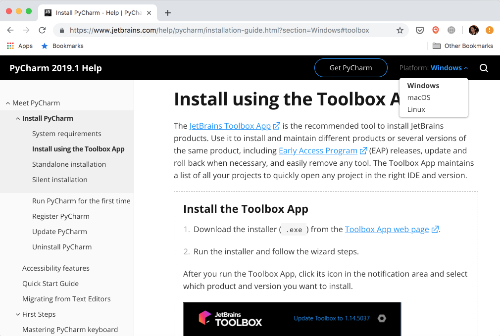
To install the Toolbox App, refer to the documentation by JetBrains. It will automatically give you the right instructions depending on your OS. In case it didn’t recognize your OS correctly, you can always find it from the drop down list on the top right section:

List of OSes in the JetBrains website

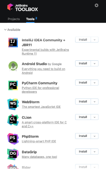
After installing, launch the app and accept the user agreement. Under the Tools tab, you’ll see a list of available products. Find PyCharm Community there and click Install:

PyCharm installed with the Toolbox app

Voilà! You have PyCharm available on your machine. If you don’t want to use the Toolbox app, then you can also do a stand-alone installation of PyCharm.

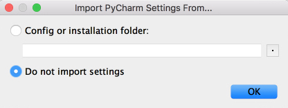
Launch PyCharm, and you’ll see the import settings popup:

PyCharm Import Settings Popup

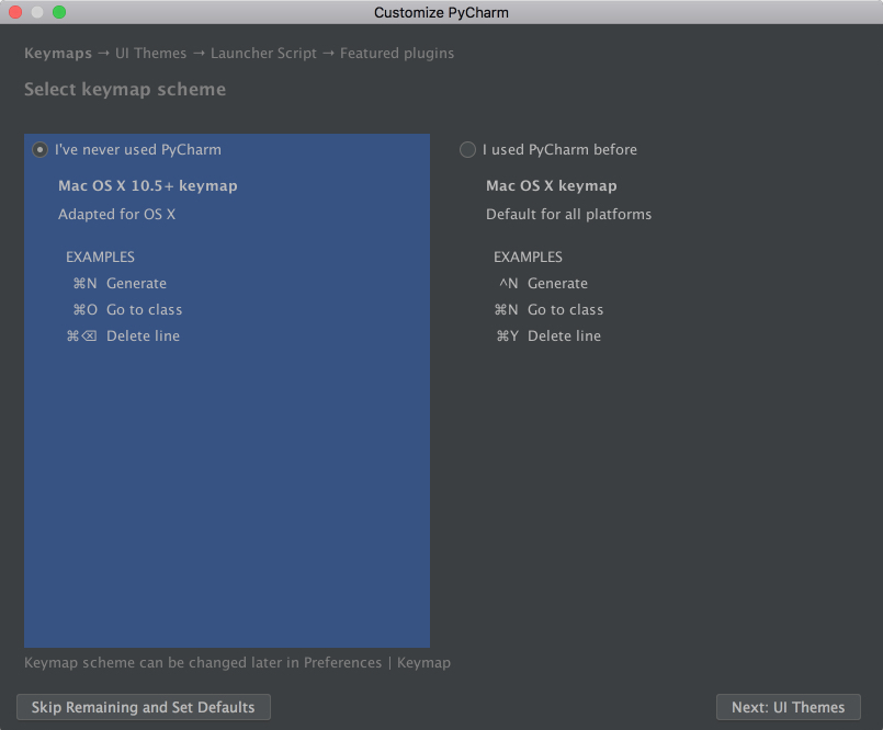
PyCharm will automatically detect that this is a fresh install and choose Do not import settings for you. Click OK, and PyCharm will ask you to select a keymap scheme. Leave the default and click Next: UI Themes on the bottom right:

PyCharm Keymap Scheme

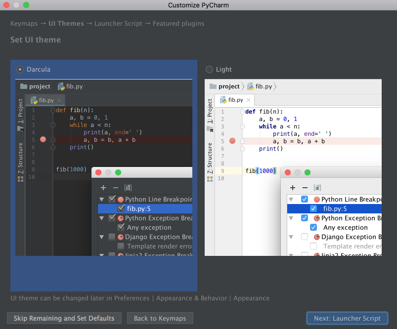
PyCharm will then ask you to choose a dark theme called Darcula or a light theme. Choose whichever you prefer and click Next: Launcher Script:

PyCharm Set UI Theme Page

I’ll be using the dark theme Darcula throughout this tutorial. You can find and install other themes as plugins, or you can also import them.

On the next page, leave the defaults and click Next: Featured plugins. There, PyCharm will show you a list of plugins you may want to install because most users like to use them. Click Start using PyCharm, and now you are ready to write some code!

Writing Code in PyCharm

In PyCharm, you do everything in the context of a project. Thus, the first thing you need to do is create one.

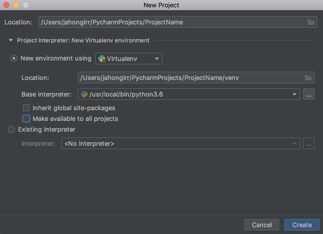
After installing and opening PyCharm, you are on the welcome screen. Click Create New Project, and you’ll see the New Project popup:

New Project in PyCharm

Specify the project location and expand the Project Interpreter drop down. Here, you have options to create a new project interpreter or reuse an existing one. Choose New environment using. Right next to it, you have a drop down list to select one of Virtualenv, Pipenv, or Conda, which are the tools that help to keep dependencies required by different projects separate by creating isolated Python environments for them.

You are free to select whichever you like, but Virtualenv is used for this tutorial. If you choose to, you can specify the environment location and choose the base interpreter from the list, which is a list of Python interpreters (such as Python2.7 and Python3.6) installed on your system. Usually, the defaults are fine. Then you have to select boxes to inherit global site-packages to your new environment and make it available to all other projects. Leave them unselected.

Click Create on the bottom right and you will see the new project created:

Project created in PyCharm

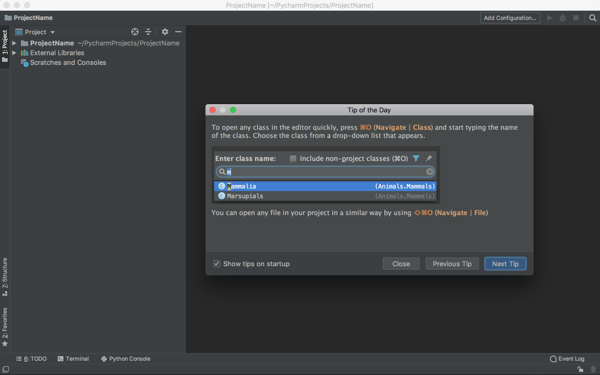
You will also see a small Tip of the Day popup where PyCharm gives you one trick to learn at each startup. Go ahead and close this popup.

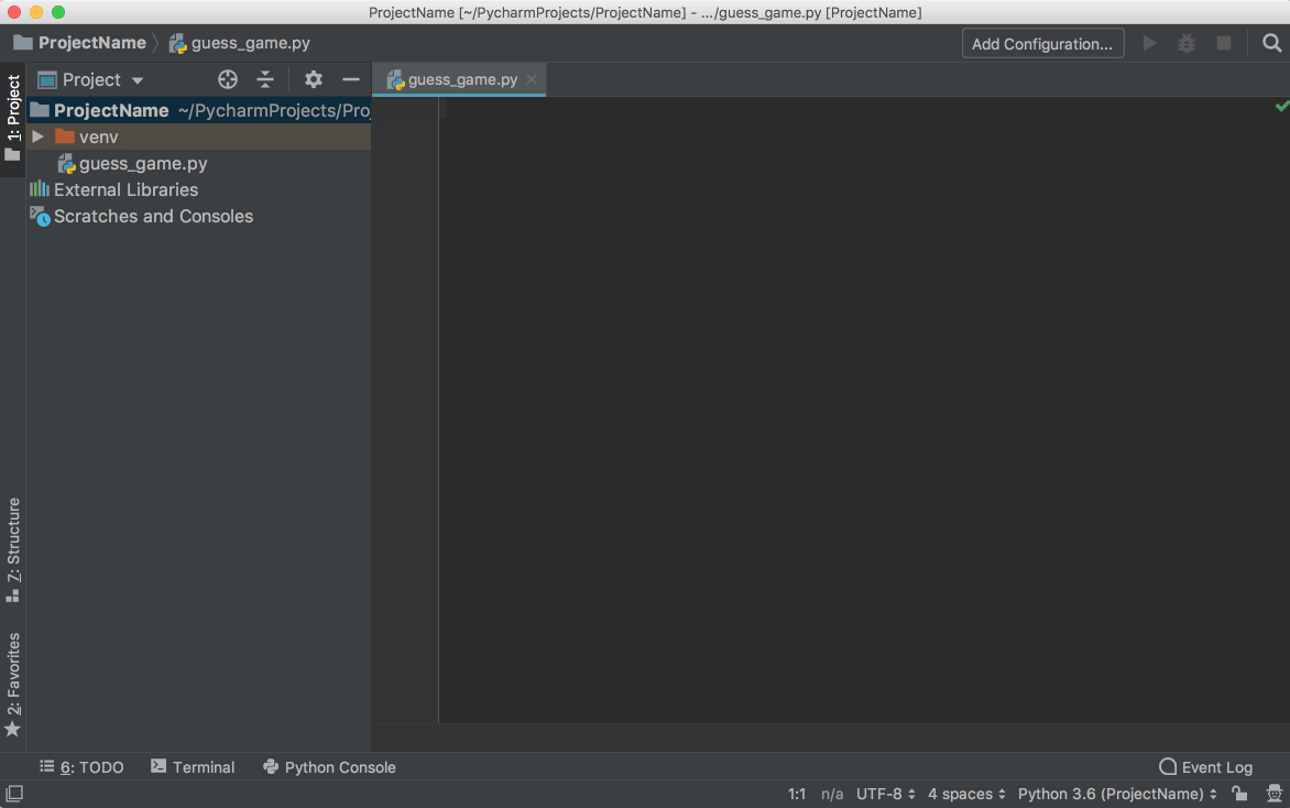
It is now time to start a new Python program. Type Cmd+N if you are on Mac or Alt+Ins if you are on Windows or Linux. Then, choose Python File. You can also select File → New from the menu. Name the new file guess_game.py and click OK. You will see a PyCharm window similar to the following:

PyCharm New File

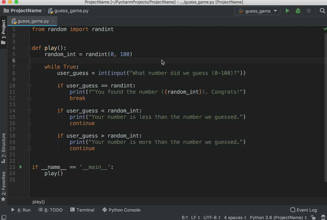
For our test code, let’s quickly code up a simple guessing game in which the program chooses a number that the user has to guess. For every guess, the program will tell if the user’s guess was smaller or bigger than the secret number. The game ends when the user guesses the number. Here’s the code for the game:

 1 fromrandomimportrandint 2  3 defplay(): 4 random_int=randint(0,100) 5  6 whileTrue: 7 user_guess=int(input("What number did we guess (0-100)?")) 8  9 ifuser_guess==randint:10 print(f"You found the number ({random_int}). Congrats!")11 break12 13 ifuser_guess<random_int:14 print("Your number is less than the number we guessed.")15 continue16 17 ifuser_guess>random_int:18 print("Your number is more than the number we guessed.")19 continue20 21 22 if__name__=='__main__':23 play()

Type this code directly rather than copying and pasting. You’ll see something like this:

Typing Guessing Game

As you can see, PyCharm provides Intelligent Coding Assistance with code completion, code inspections, on-the-fly error highlighting, and quick-fix suggestions. In particular, note how when you typed main and then hit tab, PyCharm auto-completed the whole main clause for you.

Also note how, if you forget to type if before the condition, append .if, and then hit Tab, PyCharm fixes the if clause for you. The same is true with True.while. That’s PyCharm’s Postfix completions working for you to help reduce backward caret jumps.

Running Code in PyCharm

Now that you’ve coded up the game, it’s time for you to run it.

You have three ways of running this program:

  1. Use the shortcut Ctrl+Shift+R on Mac or Ctrl+Shift+F10 on Windows or Linux.
  2. Right-click the background and choose Run ‘guess_game’ from the menu.
  3. Since this program has the __main__ clause, you can click on the little green arrow to the left of the __main__ clause and choose Run ‘guess_game’ from there.

Use any one of the options above to run the program, and you’ll see the Terminal pane appear at the bottom of the window, with your code output showing:

Running a script in PyCharm

Play the game for a little bit to see if you can find the number guessed. Pro tip: start with 50.

Debugging in PyCharm

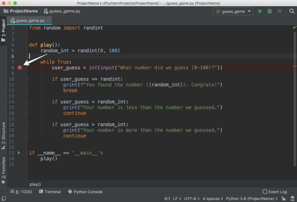
Did you find the number? If so, you may have seen something weird after you found the number. Instead of printing the congratulations message and exiting, the program seems to start over. That’s a bug right there. To discover why the program starts over, you’ll now debug the program.

First, place a breakpoint by clicking on the blank space to the left of line number 8:

Debug breakpoint in PyCharm

This will be the point where the program will be suspended, and you can start exploring what went wrong from there on. Next, choose one of the following three ways to start debugging:

  1. Press Ctrl+Shift+D on Mac or Shift+Alt+F9 on Windows or Linux.
  2. Right-click the background and choose Debug ‘guess_game’.
  3. Click on the little green arrow to the left of the __main__ clause and choose Debug ‘guess_game from there.

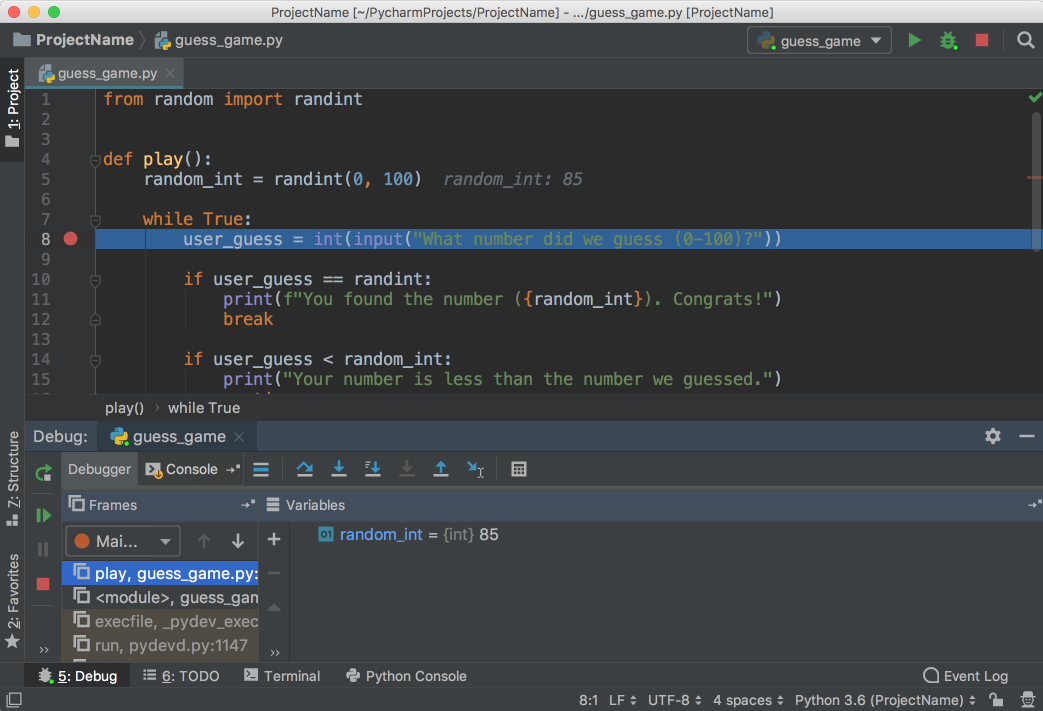
Afterwards, you’ll see a Debug window open at the bottom:

Start of debugging in PyCharm

Follow the steps below to debug the program:

  1. Notice that the current line is highlighted in blue.

  2. See that random_int and its value are listed in the Debug window. Make a note of this number. (In the picture, the number is 85.)

  3. Hit F8 to execute the current line and step over to the next one. You can also use F7 to step into the function in the current line, if necessary. As you continue executing the statements, the changes in the variables will be automatically reflected in the Debugger window.

  4. Notice that there is the Console tab right next to the Debugger tab that opened. This Console tab and the Debugger tab are mutually exclusive. In the Console tab, you will be interacting with your program, and in the Debugger tab you will do the debugging actions.

  5. Switch to the Console tab to enter your guess.

  6. Type the number shown, and then hit Enter.

  7. Switch back to the Debugger tab.

  8. Hit F8 again to evaluate the if statement. Notice that you are now on line 14. But wait a minute! Why didn’t it go to the line 11? The reason is that the if statement on line 10 evaluated to False. But why did it evaluate to False when you entered the number that was chosen?

  9. Look carefully at line 10 and notice that we are comparing user_guess with the wrong thing. Instead of comparing it with random_int, we are comparing it with randint, the function that was imported from the random package.

  10. Change it to random_int, restart the debugging, and follow the same steps again. You will see that, this time, it will go to line 11, and line 10 will evaluate to True:

Debugging Script in PyCharm

Congratulations! You fixed the bug.

Testing in PyCharm

No application is reliable without unit tests. PyCharm helps you write and run them very quickly and comfortably. By default, unittest is used as the test runner, but PyCharm also supports other testing frameworks such as pytest, nose, doctest, tox, and trial. You can, for example, enable pytest for your project like this:

  1. Open the Settings/Preferences → Tools → Python Integrated Tools settings dialog.
  2. Select pytest in the Default test runner field.
  3. Click OK to save the settings.

For this example, we’ll be using the default test runner unittest.

In the same project, create a file called calculator.py and put the following Calculator class in it:

 1 classCalculator: 2 defadd(self,a,b): 3 returna+b 4  5 defmultiply(self,a,b): 6 returna*b

PyCharm makes it very easy to create tests for your existing code. With the calculator.py file open, execute any one of the following that you like:

  • Press Shift+Cmd+T on Mac or Ctrl+Shift+T on Windows or Linux.
  • Right-click in the background of the class and then choose Go To and Test.
  • On the main menu, choose Navigate → Test.

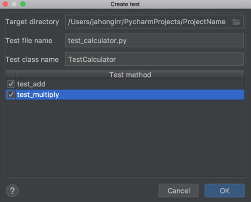
Choose Create New Test…, and you will see the following window:

Create tests in PyCharm

Leave the defaults of Target directory, Test file name, and Test class name. Select both of the methods and click OK. Voila! PyCharm automatically created a file called test_calculator.py and created the following stub tests for you in it:

 1 fromunittestimportTestCase 2  3 classTestCalculator(TestCase): 4 deftest_add(self): 5 self.fail() 6  7 deftest_multiply(self): 8 self.fail()

Run the tests using one of the methods below:

  • Press Ctrl+R on Mac or Shift+F10 on Windows or Linux.
  • Right-click the background and choose Run ‘Unittests for test_calculator.py’.
  • Click on the little green arrow to the left of the test class name and choose Run ‘Unittests for test_calculator.py’.

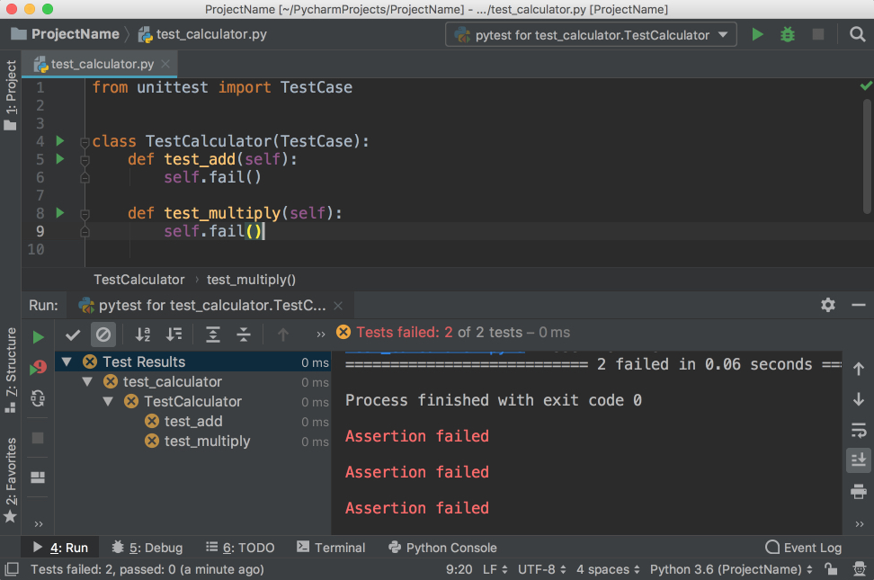
You’ll see the tests window open on the bottom with all the tests failing:

Failed tests in PyCharm

Notice that you have the hierarchy of the test results on the left and the output of the terminal on the right.

Now, implement test_add by changing the code to the following:

 1 fromunittestimportTestCase 2  3 fromcalculatorimportCalculator 4  5 classTestCalculator(TestCase): 6 deftest_add(self): 7 self.calculator=Calculator() 8 self.assertEqual(self.calculator.add(3,4),7) 9 10 deftest_multiply(self):11 self.fail()

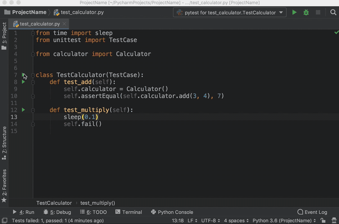
Run the tests again, and you’ll see that one test passed and the other failed. Explore the options to show passed tests, to show ignored tests, to sort tests alphabetically, and to sort tests by duration:

Running tests in PyCharm

Note that the sleep(0.1) method that you see in the GIF above is intentionally used to make one of the tests slower so that sorting by duration works.

Editing an Existing Project in PyCharm

These single file projects are great for examples, but you’ll often work on much larger projects over a longer period of time. In this section, you’ll take a look at how PyCharm works with a larger project.

To explore the project-focused features of PyCharm, you’ll use the Alcazar web framework that was built for learning purposes. To continue following along, clone the repo locally:

Clone Repo:Click here to clone the repo you'll use to explore the project-focused features of PyCharm in this tutorial.

Once you have a project locally, open it in PyCharm using one of the following methods:

  • Click File → Open on the main menu.
  • Click Open on the Welcome Screen if you are there.

After either of these steps, find the folder containing the project on your computer and open it.

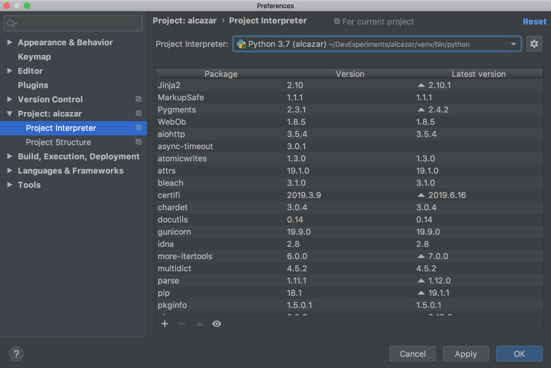
If this project contains a virtual environment, then PyCharm will automatically use this virtual environment and make it the project interpreter.

If you need to configure a different virtualenv, then open Preferences on Mac by pressing Cmd+, or Settings on Windows or Linux by pressing Ctrl+Alt+S and find the Project: ProjectName section. Open the drop-down and choose Project Interpreter:

Project interpreter in PyCharm

Choose the virtualenv from the drop-down list. If it’s not there, then click on the settings button to the right of the drop-down list and then choose Add…. The rest of the steps should be the same as when we were creating a new project.

Searching and Navigating in PyCharm

In a big project where it’s difficult for a single person to remember where everything is located, it’s very important to be able to quickly navigate and find what you looking for. PyCharm has you covered here as well. Use the project you opened in the section above to practice these shortcuts:

  • Searching for a fragment in the current file: Press Cmd+F on Mac or Ctrl+F on Windows or Linux.
  • Searching for a fragment in the entire project: Press Cmd+Shift+F on Mac or Ctrl+Shift+F on Windows or Linux.
  • Searching for a class: Press Cmd+O on Mac or Ctrl+N on Windows or Linux.
  • Searching for a file: Press Cmd+Shift+O on Mac or Ctrl+Shift+N on Windows or Linux.
  • Searching all if you don’t know whether it’s a file, class, or a code fragment that you are looking for: Press Shift twice.

As for the navigation, the following shortcuts may save you a lot of time:

  • Going to the declaration of a variable: Press Cmd on Mac or Ctrl on Windows or Linux, and click on the variable.
  • Finding usages of a class, a method, or any symbol: Press Alt+F7.
  • Seeing your recent changes: Press Shift+Alt+C or go to View → Recent Changes on the main menu.
  • Seeing your recent files: Press Cmd+E on Mac or Ctrl+E on Windows or Linux, or go to View → Recent Files on the main menu.
  • Going backward and forward through your history of navigation after you jumped around: Press Cmd+[ / Cmd+] on Mac or Ctrl+Alt+Left / Ctrl+Alt+Right on Windows or Linux.

For more details, see the official documentation.

Using Version Control in PyCharm

Version control systems such as Git and Mercurial are some of the most important tools in the modern software development world. So, it is essential for an IDE to support them. PyCharm does that very well by integrating with a lot of popular VC systems such as Git (and Github), Mercurial, Perforce and, Subversion.

Note: Git is used for the following examples.

Configuring VCS

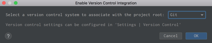
To enable VCS integration. Go to VCS → VCS Operations Popup… from the menu on the top or press Ctrl+V on Mac or Alt+` on Windows or Linux. Choose Enable Version Control Integration…. You’ll see the following window open:

Enable Version Control Integration in PyCharm

Choose Git from the drop down list, click OK, and you have VCS enabled for your project. Note that if you opened an existing project that has version control enabled, then PyCharm will see that and automatically enable it.

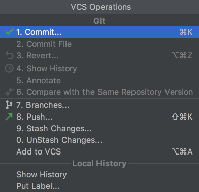
Now, if you go to the VCS Operations Popup…, you’ll see a different popup with the options to do git add, git stash, git branch, git commit, git push and more:

VCS operations in PyCharm

If you can’t find what you need, you can most probably find it by going to VCS from the top menu and choosing Git, where you can even create and view pull requests.

Committing and Conflict Resolution

These are two features of VCS integration in PyCharm that I personally use and enjoy a lot! Let’s say you have finished your work and want to commit it. Go to VCS → VCS Operations Popup… → Commit… or press Cmd+K on Mac or Ctrl+K on Windows or Linux. You’ll see the following window open:

Commit window in PyCharm

In this window, you can do the following:

  1. Choose which files to commit
  2. Write your commit message
  3. Do all kinds of checks and cleanup before commit
  4. See the difference of changes
  5. Commit and push at once by pressing the arrow to the right of the Commit button on the right bottom and choosing Commit and Push…

It can feel magical and fast, especially if you’re used to doing everything manually on the command line.

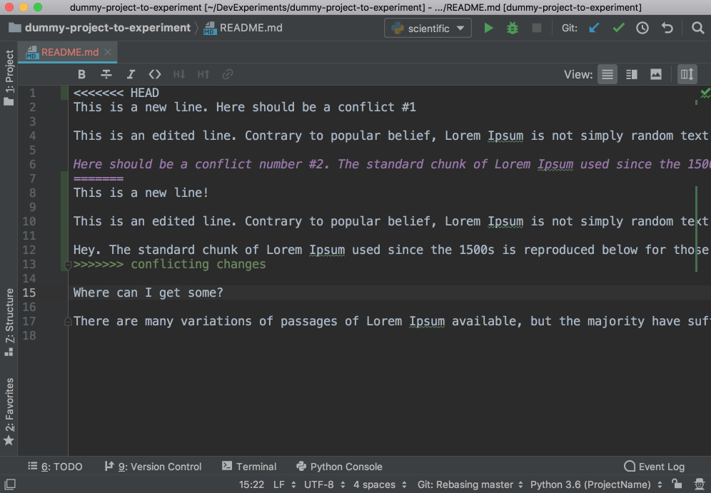
When you work in a team, merge conflicts do happen. When somebody commits changes to a file that you’re working on, but their changes overlap with yours because both of you changed the same lines, then VCS will not be able to figure out if it should choose your changes or those of your teammate. So you’ll get these unfortunate arrows and symbols:

Conflicts in PyCharm

This looks strange, and it’s difficult to figure out which changes should be deleted and which ones should stay. PyCharm to the rescue! It has a much nicer and cleaner way of resolving conflicts. Go to VCS in the top menu, choose Git and then Resolve conflicts…. Choose the file whose conflicts you want to resolve and click on Merge. You will see the following window open:
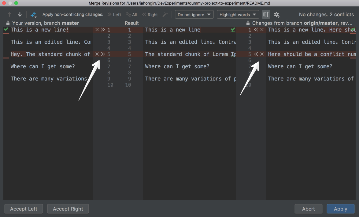
Conflict resolving windown in PyCharm

On the left column, you will see your changes. On the right one, the changes made by your teammate. Finally, in the middle column, you will see the result. The conflicting lines are highlighted, and you can see a little X and >>/<< right beside those lines. Press the arrows to accept the changes and the X to decline. After you resolve all those conflicts, click the Apply button:

Resolving Conflicts in PyCharm

In the GIF above, for the first conflicting line, the author declined his own changes and accepted those of his teammates. Conversely, the author accepted his own changes and declined his teammates’ for the second conflicting line.

There’s a lot more that you can do with the VCS integration in PyCharm. For more details, see this documentation.

Using Plugins and External Tools in PyCharm

You can find almost everything you need for development in PyCharm. If you can’t, there is most probably a plugin that adds that functionality you need to PyCharm. For example, they can:

  • Add support for various languages and frameworks
  • Boost your productivity with shortcut hints, file watchers, and so on
  • Help you learn a new programming language with coding exercises

For instance, IdeaVim adds Vim emulation to PyCharm. If you like Vim, this can be a pretty good combination.

Material Theme UI changes the appearance of PyCharm to a Material Design look and feel:

Material Theme in PyCharm

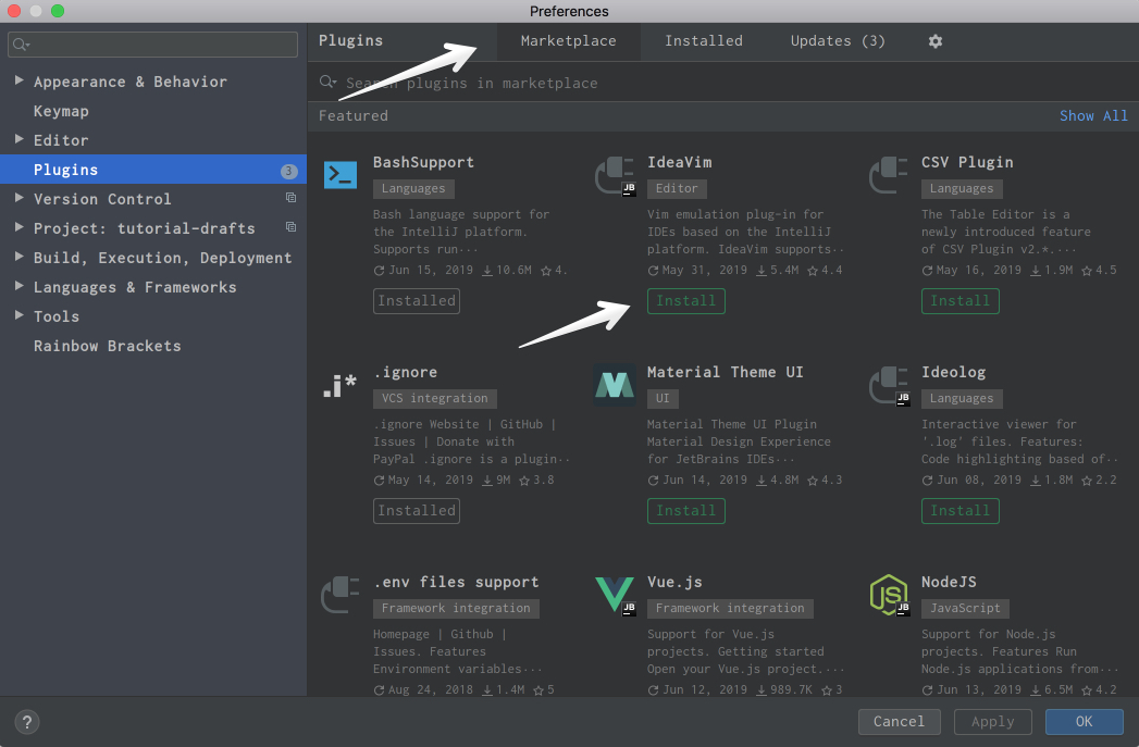
Vue.js adds support for Vue.js projects. Markdown provides the capability to edit Markdown files within the IDE and see the rendered HTML in a live preview. You can find and install all of the available plugins by going to the Preferences → Plugins on Mac or Settings → Plugins on Windows or Linux, under the Marketplace tab:

Plugin Marketplace in PyCharm

If you can’t find what you need, you can even develop your own plugin.

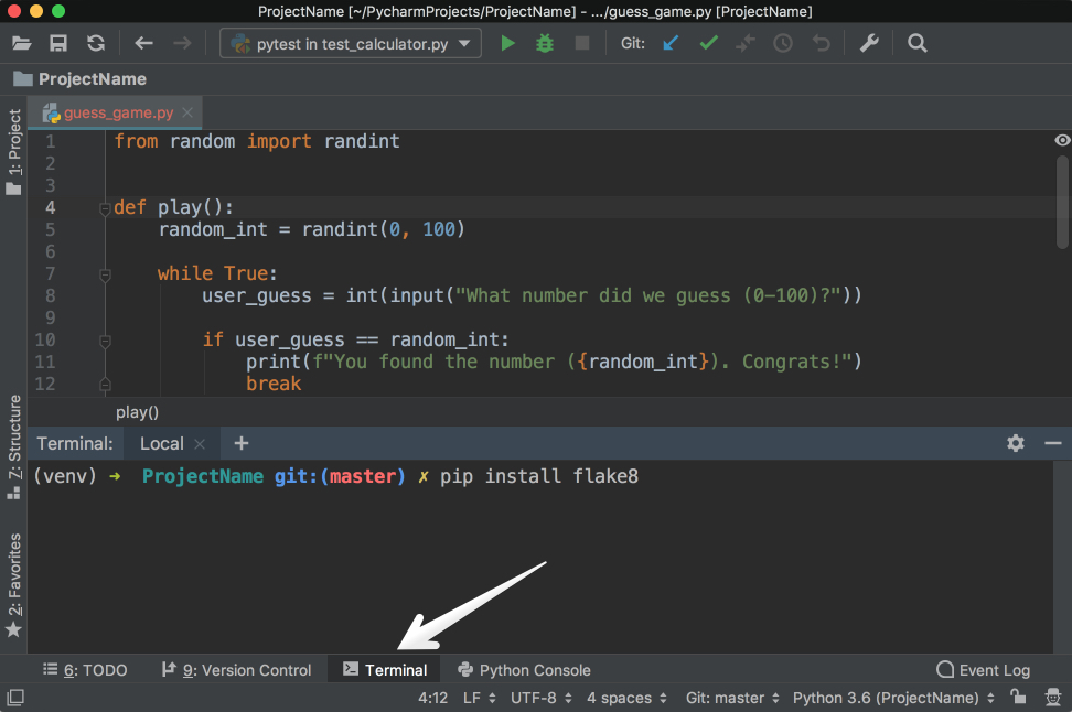
If you can’t find the right plugin and don’t want to develop your own because there’s already a package in PyPI, then you can add it to PyCharm as an external tool. Take Flake8, the code analyzer, as an example.

First, install flake8 in your virtualenv with pip install flake8 in the Terminal app of your choice. You can also use the one integrated into PyCharm:

Terminal in PyCharm

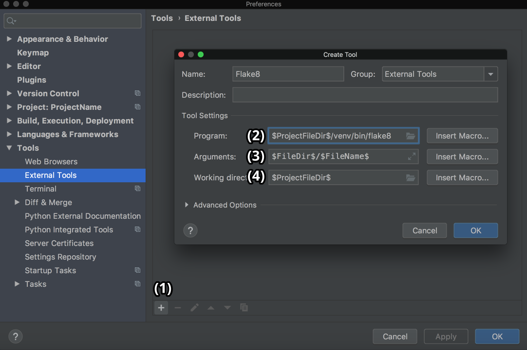
Then, go to Preferences → Tools on Mac or Settings → Tools on Windows/Linux, and then choose External Tools. Then click on the little + button at the bottom (1). In the new popup window, insert the details as shown below and click OK for both windows:

Flake8 tool in PyCharm

Here, Program (2) refers to the Flake8 executable that can be found in the folder /bin of your virtual environment. Arguments (3) refers to which file you want to analyze with the help of Flake8. Working directory is the directory of your project.

You could hardcode the absolute paths for everything here, but that would mean that you couldn’t use this external tool in other projects. You would be able to use it only inside one project for one file.

So you need to use something called Macros. Macros are basically variables in the format of $name$ that change according to your context. For example, $FileName$ is first.py when you’re editing first.py, and it is second.py when you’re editing second.py. You can see their list and insert any of them by clicking on the Insert Macro… buttons. Because you used macros here, the values will change according to the project you’re currently working on, and Flake8 will continue to do its job properly.

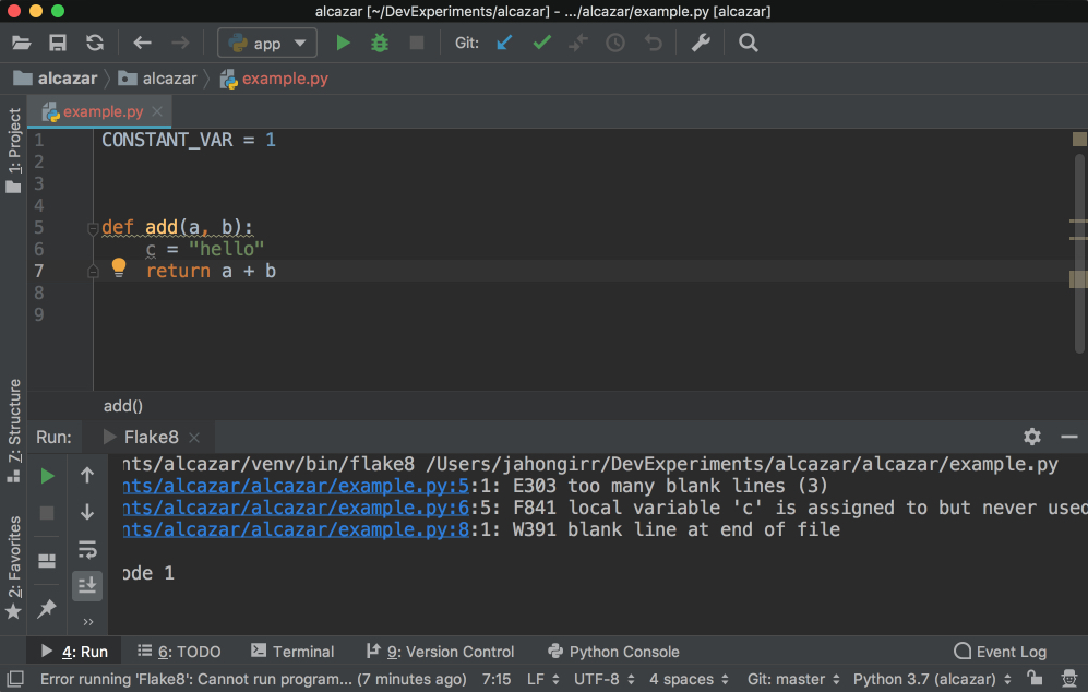
In order to use it, create a file example.py and put the following code in it:

 1 CONSTANT_VAR=1 2  3  4  5 defadd(a,b): 6 c="hello" 7 returna+b

It deliberately breaks some of the Flake8 rules. Right-click the background of this file. Choose External Tools and then Flake8. Voilà! The output of the Flake8 analysis will appear at the bottom:

Flake8 Output in PyCharm

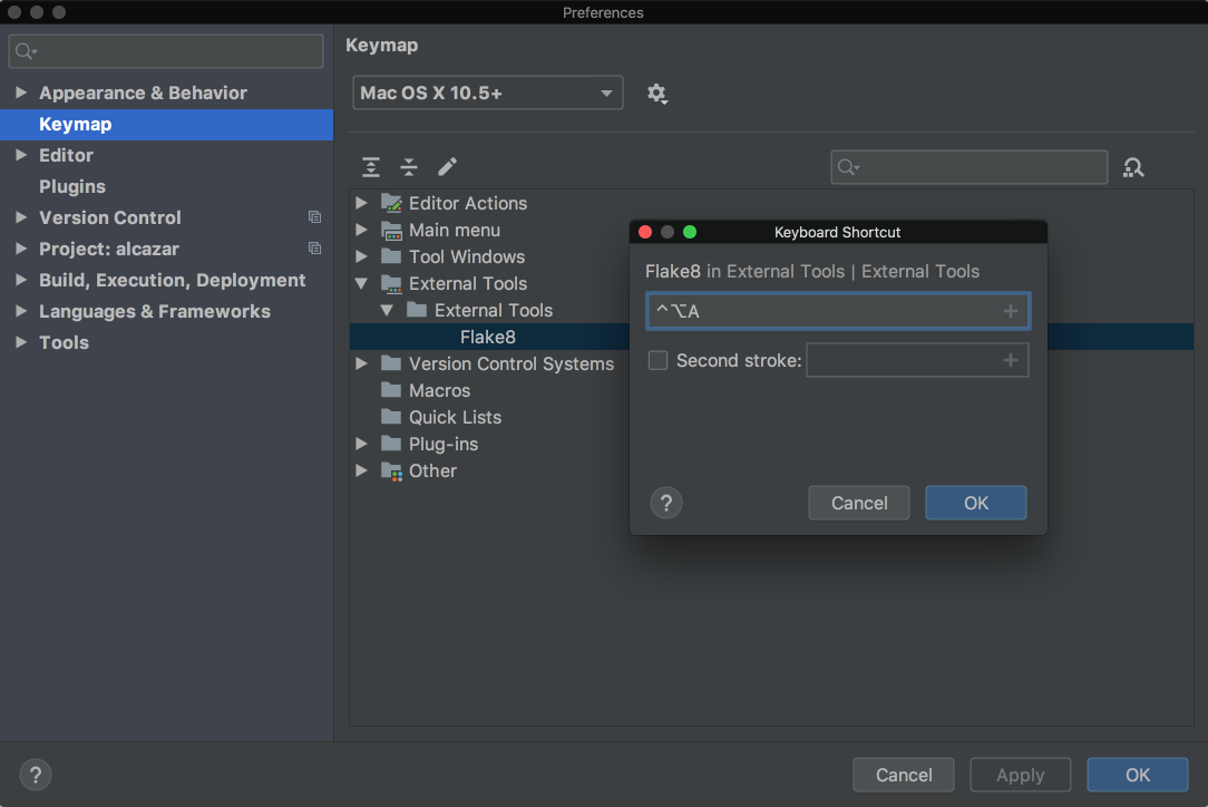
In order to make it even better, you can add a shortcut for it. Go to Preferences on Mac or to Settings on Windows or Linux. Then, go to Keymap → External Tools → External Tools. Double-click Flake8 and choose Add Keyboard Shortcut. You’ll see this window:

Add shortcut in PyCharm

In the image above, the shortcut is Ctrl+Alt+A for this tool. Add your preferred shortcut in the textbox and click OK for both windows. Now you can now use that shortcut to analyze the file you’re currently working on with Flake8.

PyCharm Professional Features

PyCharm Professional is a paid version of PyCharm with more out-of-the-box features and integrations. In this section, you’ll mainly be presented with overviews of its main features and links to the official documentation, where each feature is discussed in detail. Remember that none of the following features is available in the Community edition.

Django Support

PyCharm has extensive support for Django, one of the most popular and beloved Python web frameworks. To make sure that it’s enabled, do the following:

  1. Open Preferences on Mac or Settings on Windows or Linux.
  2. Choose Languages and Frameworks.
  3. Choose Django.
  4. Check the checkbox Enable Django support.
  5. Apply changes.

Now that you’ve enabled Django support, your Django development journey will be a lot easier in PyCharm:

  • When creating a project, you’ll have a dedicated Django project type. This means that, when you choose this type, you’ll have all the necessary files and settings. This is the equivalent of using django-admin startproject mysite.
  • You can run manage.py commands directly inside PyCharm.
  • Django templates are supported, including:
    • Syntax and error highlighting
    • Code completion
    • Navigation
    • Completion for block names
    • Completion for custom tags and filters
    • Quick documentation for tags and filters
    • Capability to debug them
  • Code completion in all other Django parts such as views, URLs and models, and code insight support for Django ORM.
  • Model dependency diagrams for Django models.

For more details on Django support, see the official documentation.

Database Support

Modern database development is a complex task with many supporting systems and workflows. That’s why JetBrains, the company behind PyCharm, developed a standalone IDE called DataGrip for that. It’s a separate product from PyCharm with a separate license.

Luckily, PyCharm supports all the features that are available in DataGrip through a plugin called Database tools and SQL, which is enabled by default. With the help of it, you can query, create and manage databases whether they’re working locally, on a server, or in the cloud. The plugin supports MySQL, PostgreSQL, Microsoft SQL Server, SQLite, MariaDB, Oracle, Apache Cassandra, and others. For more information on what you can do with this plugin, check out the comprehensive documentation on the database support.

Thread Concurrency Visualization

Django Channels, asyncio, and the recent frameworks like Starlette are examples of a growing trend in asynchronous Python programming. While it’s true that asynchronous programs do bring a lot of benefits to the table, it’s also notoriously hard to write and debug them. In such cases, Thread Concurrency Visualization can be just what the doctor ordered because it helps you take full control over your multi-threaded applications and optimize them.

Check out the comprehensive documentation of this feature for more details.

Profiler

Speaking of optimization, profiling is another technique that you can use to optimize your code. With its help, you can see which parts of your code are taking most of the execution time. A profiler runs in the following order of priority:

  1. vmprof
  2. yappi
  3. cProfile

If you don’t have vmprof or yappi installed, then it’ll fall back to the standard cProfile. It’s well-documented, so I won’t rehash it here.

Scientific Mode

Python is not only a language for general and web programming. It also emerged as the best tool for data science and machine learning over these last years thanks to libraries and tools like NumPy, SciPy, scikit-learn, Matplotlib, Jupyter, and more. With such powerful libraries available, you need a powerful IDE to support all the functions such as graphing and analyzing those libraries have. PyCharm provides everything you need as thoroughly documented here.

Remote Development

One common cause of bugs in many applications is that development and production environments differ. Although, in most cases, it’s not possible to provide an exact copy of the production environment for development, pursuing it is a worthy goal.

With PyCharm, you can debug your application using an interpreter that is located on the other computer, such as a Linux VM. As a result, you can have the same interpreter as your production environment to fix and avoid many bugs resulting from the difference between development and production environments. Make sure to check out the official documentation to learn more.

Conclusion

PyCharm is one of best, if not the best, full-featured, dedicated, and versatile IDEs for Python development. It offers a ton of benefits, saving you a lot of time by helping you with routine tasks. Now you know how to be productive with it!

In this article, you learned about a lot, including:

  • Installing PyCharm
  • Writing code in PyCharm
  • Running your code in PyCharm
  • Debugging and testing your code in PyCharm
  • Editing an existing project in PyCharm
  • Searching and navigating in PyCharm
  • Using Version Control in PyCharm
  • Using Plugins and External Tools in PyCharm
  • Using PyCharm Professional features, such as Django support and Scientific mode

If there’s anything you’d like to ask or share, please reach out in the comments below. There’s also a lot more information at the PyCharm website for you to explore.

Clone Repo:Click here to clone the repo you'll use to explore the project-focused features of PyCharm in this tutorial.


[ Improve Your Python With 🐍 Python Tricks 💌 – Get a short & sweet Python Trick delivered to your inbox every couple of days. >> Click here to learn more and see examples ]

Ruslan Spivak: Let’s Build A Simple Interpreter. Part 17: Call Stack and Activation Records

$
0
0

You may have to fight a battle more than once to win it.” — Margaret Thatcher

In 1968 during the Mexico City Summer Olympics, a marathon runner named John Stephen Akhwari found himself thousands miles away from his home country of Tanzania, in East Africa. While running the marathon at the high altitude of Mexico City he got hit by other athletes jockeying for position and fell to the ground, badly wounding his knee and causing a dislocation. After receiving medical attention, instead of pulling out of the competition after such a bad injury, he stood up and continued the race.

Mamo Wolde of Ethiopia, at 2:20:26 into the race, crossed the finish line in first place. More than an hour later at 3:25:27, after the sun had set, Akhwari, hobbling, with a bloody leg and his bandages dangling and flapping in the wind, crossed the finish line, in last place.

When a small crowd saw Akhwari crossing the line, they cheered him in disbelief, and the few remaining reporters rushed onto the track to ask him why he continued to run the race with his injuries. His response went down in history: “My country did not send me 5,000 miles to start the race. They sent me 5,000 miles to finish the race.”

This story has since inspired many athletes and non-athletes alike. You might be thinking at this point, “That’s great, it’s an inspiring story, but what does it have to do with me?” The main message for you and me is this: “Keep going!” This has been a long series spun over a long period of time and at times it may feel daunting to go along with it, but we’re approaching an important milestone in the series, so we need to keep going.

Okay, let’s get to it!

We have a couple of goals for today:

  1. Implement a new memory system that can support programs, procedure calls, and function calls.

  2. Replace the interpreter’s current memory system, represented by the GLOBAL_MEMORY dictionary, with the new memory system.

Let’s start by answering the following questions:

  1. What is a memory system?

  2. Why do we need a new memory system?

  3. What does the new memory system look like?

  4. Why would we want to replace the GLOBAL_MEMORY dictionary?


1. What is a memory system?

To put it simply, it is a system for storing and accessing data in memory. At the hardware level, it is the physical memory (RAM) where values are stored at particular physical addresses. At the interpreter level, because our interpreter stores values according to their variable names and not physical addresses, we represent memory with a dictionary that maps names to values. Here is a simple demonstration where we store the value of 7 by the variable name y, and then immediately access the value associated with the name y:

>>> GLOBAL_MEMORY = {}
>>>
>>> GLOBAL_MEMORY['y'] = 7   # store value by name
>>>
>>> GLOBAL_MEMORY['y']       # access value by name
7
>>>


We’ve been using this dictionary approach to represent global memory for a while now. We’ve been storing and accessing variables at the PROGRAM level (the global level) using the GLOBAL_MEMORY dictionary. Here are the parts of the interpreter concerned with the “memory” creation, handling assignments of values to variables in memory and accessing values by their names:

classInterpreter(NodeVisitor):def__init__(self,tree):self.tree=treeself.GLOBAL_MEMORY={}defvisit_Assign(self,node):var_name=node.left.valuevar_value=self.visit(node.right)self.GLOBAL_MEMORY[var_name]=var_valuedefvisit_Var(self,node):var_name=node.valuevar_value=self.GLOBAL_MEMORY.get(var_name)returnvar_value

Now that we’ve described how we currently represent memory in our interpreter, let’s find out an answer to the next question.

2. Why do we need a new memory system for our interpreter?

It turns out that having just one dictionary to represent global memory is not enough to support procedure and function calls, including recursive calls.

To support nested calls, and a special case of nested calls, recursive calls, we need multiple dictionaries to store information about each procedure and function invocation. And we need those dictionaries organized in a particular way. That’s the reason we need a new memory system. Having this memory system in place is a stepping-stone for executing procedure calls, which we will implement in future articles.

3. What does the new memory system look like?

At its core, the new memory system is a stack data structure that holds dictionary-like objects as its elements. This stack is called the “call stack” because it’s used to track what procedure/function call is being currently executed. The call stack is also known as the run-time stack, execution stack, program stack, or just “the stack”. The dictionary-like objects that the call stack holds are called activation records. You may know them by another name: “stack frames”, or just “frames”.

Let’s go into more detail about the call stack and activation records.

What is a stack? A stack is a data structure that is based on a “last-in-first-out” policy (LIFO), which means that the most recent item added to the stack is the first one that comes out. It’s like a collection of plates where you put (“push”) a plate on the top of the plate stack and, if you need to take a plate, you take one off the top of the plate stack (you “pop” the plate):

Our stack implementation will have the following methods:

- push (to push an item onto the stack)

- pop (to pop an item off the stack)

- peek (to return an item at the top of the stack without removing it)


And by our convention our stack will be growing upwards:

How would we implement a stack in code? A very basic implementation could look like this:

classStack:def__init__(self):self.items=[]defpush(self,item):self.items.append(item)defpop(self):returnself.items.pop()defpeek(self):returnself.items[-1]

That’s pretty much how our call stack implementation will look as well. We’ll change some variable names to reflect the fact that the call stack will store activation records and add a __str__() method to print the contents of the stack:

classCallStack:def__init__(self):self._records=[]defpush(self,ar):self._records.append(ar)defpop(self):returnself._records.pop()defpeek(self):returnself._records[-1]def__str__(self):s='\n'.join(repr(ar)forarinreversed(self._records))s=f'CALL STACK\n{s}\n'returnsdef__repr__(self):returnself.__str__()

The __str__() method generates a string representation of the contents of the call stack by iterating over activation records in reverse order and concatenating a string representation of each record to produce the final result. The __str__() method prints the contents in the reverse order so that the standard output shows our stack growing up.

Now, what is an activation record? For our purposes, an activation record is a dictionary-like object for maintaining information about the currently executing invocation of a procedure or function, and also the program itself. The activation record for a procedure invocation, for example, will contain the current values of its formal parameters and its local variables.

Let’s take a look at how we will represent activation records in code:

classARType(Enum):PROGRAM='PROGRAM'classActivationRecord:def__init__(self,name,type,nesting_level):self.name=nameself.type=typeself.nesting_level=nesting_levelself.members={}def__setitem__(self,key,value):self.members[key]=valuedef__getitem__(self,key):returnself.members[key]defget(self,key):returnself.members.get(key)def__str__(self):lines=['{level}: {type} {name}'.format(level=self.nesting_level,type=self.type.value,name=self.name,)]forname,valinself.members.items():lines.append(f'   {name:<20}: {val}')s='\n'.join(lines)returnsdef__repr__(self):returnself.__str__()

There are a few things worth mentioning:

a. The ActivationRecord class constructor takes three parameters:

  • the name of the activation record (AR for short); we’ll use a program name as well as a procedure/function name as the name for the corresponding AR

  • the type of the activation record (for example, PROGRAM); these are defined in a separate enumeration class called ARType (activation record type)

  • the nesting_level of the activation record; the nesting level of an AR corresponds to the scope level of the respective procedure or function declaration plus one; the nesting level will always be set to 1 for programs, which you’ll see shortly

b. The members dictionary represents memory that will be used for keeping information about a particular invocation of a routine. We’ll cover this in more detail in the next article

c. The ActivationRecord class implements special __setitem__() and __getitem__() methods to give activation record objects a dictionary-like interface for storing key-value pairs and for accessing values by keys: ar[‘x’] = 7 and ar[‘x’]

d. The get() method is another way to get a value by key, but instead of raising an exception, the method will return None if the key doesn’t exist in the members dictionary yet.

e. The __str__() method returns a string representation of the contents of an activation record

Let’s see the call stack and activation records in action using a Python shell:

>>>fromspiimportCallStack,ActivationRecord,ARType>>>stack=CallStack()>>>stackCALLSTACK>>>ar=ActivationRecord(name='Main',type=ARType.PROGRAM,nesting_level=1)>>>>>>ar1:PROGRAMMain>>>>>>ar['y']=7>>>>>>ar1:PROGRAMMainy:7>>>>>>stackCALLSTACK>>>stack.push(ar)>>>>>>stackCALLSTACK1:PROGRAMMainy:7>>>


In the picture below, you can see the description of the contents of the activation record from the interactive session above:

AR:Main1 denotes an activation record for the program named Main at nesting level 1.

Now that we’ve covered the new memory system, let’s answer the following question.


4. Why would we want to replace the GLOBAL_MEMORY dictionary with the call stack?

The reason is to simplify our implementation and to have unified access to global variables defined at the PROGRAM level as well as to procedure and function parameters and their local variables.

In the next article we’ll see how it all fits together, but for now let’s get to the Interpreter class changes where we put the call stack and activation records described earlier to good use.


Here are all the interpreter changes we’re going to make today:

1. Replace the GLOBAL_MEMORY dictionary with the call stack

2. Update the visit_Program method to use the call stack to push and pop an activation record that will hold the values of global variables

3. Update the visit_Assign method to store a key-value pair in the activation record at the top of the call stack

4. Update the visit_Var method to access a value by its name from the activation record at the top of the call stack

5. Add a log method and update the visit_Program method to use it to print the contents of the call stack when interpreting a program

Let’s get started, shall we?

1. First things first, let’s replace the GLOBAL_MEMORY dictionary with our call stack implementation. All we need to do is change the Interpreter constructor from this:

classInterpreter(NodeVisitor):def__init__(self,tree):self.tree=treeself.GLOBAL_MEMORY={}

to this:

classInterpreter(NodeVisitor):def__init__(self,tree):self.tree=treeself.call_stack=CallStack()

2. Now, let’s update the visit_Program method:

Old code:

defvisit_Program(self,node):self.visit(node.block)

New code:

defvisit_Program(self,node):program_name=node.namear=ActivationRecord(name=program_name,type=ARType.PROGRAM,nesting_level=1,)self.call_stack.push(ar)self.visit(node.block)self.call_stack.pop()

Let’s unpack what’s going on in the updated method above:

  • First, we create an activation record, giving it the name of the program, the PROGRAM type, and the nesting level 1

  • Then we push the activation record onto the call stack; we do this before anything else so that the rest of the interpreter can use the call stack with the single activation record at the top of the stack to store and access global variables

  • Then we evaluate the body of the program as usual. Again, as our interpreter evaluates the body of the program, it uses the activation record at the top of the call stack to store and access global variables

  • Next, right before exiting the visit_Program method, we pop the activation record off the call stack; we don’t need it anymore because at this point the execution of the program by the interpreter is over and we can safely discard the activation record that is no longer used

3. Up next, let’s update the visit_Assign method to store a key-value pair in the activation record at the top of the call stack:

Old code:

defvisit_Assign(self,node):var_name=node.left.valuevar_value=self.visit(node.right)self.GLOBAL_MEMORY[var_name]=var_value

New code:

defvisit_Assign(self,node):var_name=node.left.valuevar_value=self.visit(node.right)ar=self.call_stack.peek()ar[var_name]=var_value

In the code above we use the peek() method to get the activation record at the top of the stack (the one that was pushed onto the stack by the visit_Program method) and then use the record to store the value var_value using var_name as a key.

4. Next, let’s update the visit_Var method to access a value by its name from the activation record at the top of the call stack:

Old code:

defvisit_Var(self,node):var_name=node.valuevar_value=self.GLOBAL_MEMORY.get(var_name)returnvar_value

New code:

defvisit_Var(self,node):var_name=node.valuear=self.call_stack.peek()var_value=ar.get(var_name)returnvar_value

Again as you can see, we use the peek() method to get the top (and only) activation record - the one that was pushed onto the stack by the visit_Program method to hold all the global variables and their values - and then get a value associated with the var_name key.

5. And the last change in the Interpreter class that we’re going to make is to add a log method and use the log method to print the contents of the call stack when the interpreter evaluates a program:

deflog(self,msg):if_SHOULD_LOG_STACK:print(msg)defvisit_Program(self,node):program_name=node.nameself.log(f'ENTER: PROGRAM {program_name}')ar=ActivationRecord(name=program_name,type=ARType.PROGRAM,nesting_level=1,)self.call_stack.push(ar)self.log(str(self.call_stack))self.visit(node.block)self.log(f'LEAVE: PROGRAM {program_name}')self.log(str(self.call_stack))self.call_stack.pop()

The messages will be logged only if the global variable _SHOULD_LOG_STACK is set to true. The variable’s value will be controlled by the “—stack” command line option. First, let’s update the main function and add the “—stack” command line option to turn the logging of the call stack contents on and off:

defmain():parser=argparse.ArgumentParser(description='SPI - Simple Pascal Interpreter')parser.add_argument('inputfile',help='Pascal source file')parser.add_argument('--scope',help='Print scope information',action='store_true',)parser.add_argument('--stack',help='Print call stack',action='store_true',)args=parser.parse_args()global_SHOULD_LOG_SCOPE,_SHOULD_LOG_STACK_SHOULD_LOG_SCOPE,_SHOULD_LOG_STACK=args.scope,args.stack


Now, let’s take our updated interpreter for a test drive. Download the interpreter from GitHub and run it with the -h command line option to see available command line options:

$ python spi.py -h
usage: spi.py [-h][--scope][--stack] inputfile

SPI - Simple Pascal Interpreter

positional arguments:
  inputfile   Pascal source file

optional arguments:
  -h, --help  show this help message and exit
  --scope     Print scope information
  --stack     Print call stack

Download the following sample program from GitHub or save it to file part17.pas

programMain;varx,y:integer;begin{ Main }y:=7;x:=(y+3)*3;end.{ Main }

Run the interpreter with the part17.pas file as its input file and the “—stack” command line option to see the contents of the call stack as the interpreter executes the source program:

$ python spi.py part17.pas --stack
ENTER: PROGRAM Main
CALL STACK
1: PROGRAM Main


LEAVE: PROGRAM Main
CALL STACK
1: PROGRAM Main
   y                   : 7
   x                   : 30


Mission accomplished! We have implemented a new memory system that can support programs, procedure calls, and function calls. And we’ve replaced the interpreter’s current memory system, represented by the GLOBAL_MEMORY dictionary, with the new system based on the call stack and activation records.


That’s all for today. In the next article we’ll extend the interpreter to execute procedure calls using the call stack and activation records. This will be a huge milestone for us. So stay tuned and see you next time!


Resources used in preparation for this article (some links are affiliate links):

  1. Language Implementation Patterns: Create Your Own Domain-Specific and General Programming Languages (Pragmatic Programmers)
  2. Writing Compilers and Interpreters: A Software Engineering Approach
  3. Programming Language Pragmatics, Fourth Edition
  4. Lead with a Story
  5. A Wikipedia article on John Stephen Akhwari

Stack Abuse: Introduction to the Python Pyramid Framework

$
0
0

Introduction

In this tutorial, we're going to learn how to use the Pyramid framework in Python. It is an open source web development framework which uses the Model-View-Controller (MVC) architecture pattern and is based on Web Server Gateway Interface (WSGI). The Pyramid framework has a lot of useful add-on packages that make web development a lot more convenient. Some other popular alternatives for web development in Python include Django and Flask.

Prerequisites

You need to have basic knowledge of HTML for this tutorial. If you do not have any prior experience with it, do not worry about it, you can still follow this tutorial and understand how Pyramid works, but to develop real world web applications you will have to go back and learn HTML.

Architecture

Before we move on and see the code, let's first understand WSGI and MVC.

WSGI is basically a standard which defines the way in which a Python based web application interacts with a server. It governs the process of sending requests to a server, and receiving responses from a server.

MVC is an architectural pattern which modularizes your application; the model contains the data and business logic of your application, the view displays the relevant information to the user, and the controller is responsible for the interaction between the model and the view.

Google Maps is a perfect example of the MVC architecture. When we use the route-finding feature in Google Maps, the model contains the code for the algorithm which finds the shortest path from location A to location B, the view is the screen that is shown to you containing the map labeled with the route, and the controller contains the code that uses the shortest path found by the model and displays it to the user through the view. You can also view controller, as the code which receives a request from the view (by the user), forwards it to the model to generate a response, and then displays the response from the model back to the user through a view.

Besides WSGI and MVC, there are two more terms that you should be familiar with, which are "routes" and "scripts". Routes allow your website to be divided into different webpages, with each webpage performing a different function.

Let's consider Facebook as an example. If you wish to view your messages, a new webpage with a different view is opened up for that, if you wish to view your own profile, a new webpage is opened for that, but they are all connected to your main website. That's done through routes. Each time you click on a button or link, you are redirected to a new webpage as specified by the routes in our application.

As for scripts, they simply include configuration settings for our application, and help in managing it.

We will learn more about all these terms when we create a basic web application using Pyramid. So, let's begin.

Installation

Whenever we develop a web application that is to be deployed online, it is always considered a good practice to make a virtual environment first. The virtual environment contains all the libraries, or frameworks and all the other dependencies that are necessary for running the web app. This way, when you deploy your app to a server, you can simply re-install all those libraries on the server, for your application to run smoothly.

Let's create a virtual environment before we move forward. Install virtual environment module by running the command below in your terminal:

$ pip install virtualenv

To test that your installation was successful, run the following command:

$ virtualenv --version

If you see a version number printed to the console then the installation was successful (or virtualenv was already installed on your system).

To create a virtual environment, first navigate to the folder where you wish to create it, and then run the following command:

$ virtualenv myvenv

Note: You can name your virtual environment anything you want. Here we're using "myenv" for demonstration purposes only.

The last step is to activate your virtual environment. On Mac, run the following command in the terminal:

$ source myvenv/bin/activate

On a Windows machine, you can activate the environment with the following command:

'Installation folder'\myvenv\Scripts\activate.bat

Now that you have your virtual environment set up, let's install Pyramid in it. We will use the pip package manager for that:

$ pip install pyramid

Note: When you are done with working with the application and wish to deactivate your virtual environment, run the following command in the terminal:

$ deactivate

Coding Exercise

In this section, we will start off by coding a skeleton app to understand how the Pyramid apps are structured and how they communicate at a basic level. After that, we will see how to create applications with multiple views.

A Simple Example of Python Pyramid

# intro.py
# Import necessary functions to run our web app

from wsgiref.simple_server import make_server
from pyramid.config import Configurator
from pyramid.response import Response

# This function receives a request from the user, and returns a response
def intro(request):
    return Response('Hi, My name is Junaid Khalid')

# This function will start a server on our computer (localhost), define the
# routes for our application, and also add a view to be shown to the user
def main():
    with Configurator() as config:

        config.add_route('intro', '/')
        config.add_view(intro, route_name='intro')
        application = config.make_wsgi_app()

    # 8000 is the port number through which the requests of our app will be served
    server = make_server('0.0.0.0', 8000, application)
    server.serve_forever()

main()

Note: The Configurator module is being used to connect a particular view to a specific route. For instance, on Facebook, the "My Profile" view would be different than the "News Feed" view, and they both have different URLs as well. This is exactly what a configurator does; connecting a specific URL/route to a particular view.

Then make_server methods is used to run our application on a local HTTP server on our machine, with an assigned port number.

The intro function is used to process the requests received from the user, process them, and return the response to the view. Any processing of the request before sending a response, can be done inside this function.

To run the above application on your workstation, go to the terminal and run the .py file we just created:

$ python3 intro.py

In my case, the filename is intro.py, but yours could be different depending on what you decided to name it.

Then open any web browser on your PC, and go to this address: http://localhost:8000. You should see a webpage with "Hi, My name is Junaid Khalid" written in a very aesthetically displeasing way. To make it look more pleasant, you can return HTML code as a response as well. For a simple example, let's edit intro function:

def intro(request):
    return Response('<h2 style="text-align: center; font-family: verdana; color: blue;">Hi, My name is Junaid Khalid.</h2>')

Replace the intro function with the one above, and see the output now. A lot better, right? This was just an example. You can make it a lot better.

Note: When you make any change in the code, the server is not automatically going to log that. You will have to stop the server, and then restart it to see your changes take effect. To do that, open your terminal where the server is running and press Control+C, this will terminate the server. Then you can restart your server as usual to see the changes.

Separating and Displaying Multiple Views

In this section, we will add a few more views as well as remove our views from the main file (i.e. 'intro.py' file), and put them all in a new separate file ('all_views.py'). This will modularize our code, make it look cleaner, and will also allow us to add new views more easily. So, let's do it.

# all_views.py
# Import necessary functions to run our web app
from pyramid.compat import escape
from pyramid.response import Response
from pyramid.view import view_config

# view_config functions tells Pyramid which route's view is going to be defined in the function that follows
# the name of the function does not matter, you can name it whatever you like

@view_config(route_name='intro')
def home_page(request):
    header = '<h2 style="text-align: center;">Home Page</h2>'
    body = '<br><br><p style="text-align: center; font-family: verdana; color: blue;">Hi, My name is Junaid Khalid.</p>'
    body += '<p style="text-align: center; font-family: verdana;"> This is my portfolio website.</p>'
    footer = '<p style="text-align: center; font-family: verdana;">Checkout my <a href="/jobs">previous jobs</a>.</p>'

    # In the 'a' tag, notice that the href contains '/jobs', this route will be defined in the intro.py file
    # It is simply telling the view to navigate to that route, and run whatever code is in that view

    return Response(header + body + footer)

@view_config(route_name='jobs')
def job_history(request):
    header = '<h2 style="text-align: center;">Job History</h2>'
    job1 = '<p style="text-align: center; font-family: verdana;">Jr. Software Developer at XYZ</p>'

    return Response(header + job1)

Note: At the beginner level, you can write the HTML code by following the strategy used above i.e. declare tags in different variables and simply concatenate them when sending back the response. At some point you'll likely want to use a templating engine, like Jinja to make HTML generation much simpler.

Our application won't run just yet, we need to edit the intro.py file as well.

# intro.py
# Import necessary functions to run our web app

from wsgiref.simple_server import make_server
from pyramid.config import Configurator
from pyramid.response import Response

def main():
    with Configurator() as config:
        # In add_route function, the first parameter defines the name of the route
        # and the second parameter defines the 'route' or the page location
        config.add_route('intro', '/')
        config.add_route('jobs', '/jobs')

        # The scan function scans our project directory for a file named all_views.py
        # and connects the routes we provided above with their relevant views
        config.scan('all_views')

        application = config.make_wsgi_app()

    # The following lines of code configure and start a server which hosts our
    # website locally (i.e. on our computer)
    server = make_server('0.0.0.0', 8000, application)
    server.serve_forever()

main()

As you can see, we have removed the code for our previous view. If we had declared all these views in a single file, the file would have looked a lot more cluttered. Both files look very clean now, and each file now serves a single purpose. Let's see what our web app looks like right now.

Output:

In the image above, we can see our home page. It is located at the route 'http://localhost:8000'. It does not look very aesthetically pleasing, but as stated at the start of the tutorial, this was not our aim anyways. If we want to make it look aesthetic, we can add a lot of styling to it using HTML style attribute, or CSS, or use templates from Bootstrap.

Moving on, you can also see a hyperlink which has been named 'previous jobs'. Clicking that would take you to a new webpage with a different route. We will see the output of that in the next image.

Output:

The above image shows our Jobs page. It is located at the route http://localhost:8000/jobs. We specified this route in our 'intro.py' file. I have only added one job to show as an example.

Conclusion

Pyramid is a Python based Web Development Framework to build web apps with ease. In this tutorial, we learned how to install Pyramid inside a virtual environment and make a basic Web Application using Pyramid which runs on a locally created server on our computer.

If you would like to go into more details, visit Pyramid's documentation - it is quite elaborate and beginner friendly.

Viewing all 22871 articles
Browse latest View live


<script src="https://jsc.adskeeper.com/r/s/rssing.com.1596347.js" async> </script>