Quantcast
Channel: Planet Python
Viewing all 22871 articles
Browse latest View live

PSF GSoC students blogs: Panda3D iOS Support - A Postmortem

$
0
0

Hi everyone!

Well, it appears that this is the end of the line when it comes to my GSoC portion of my work. I got a huge amount of work done and am extremely proud of it, and I can't wait to continue working on this project in the coming months and make it the best it can be. This blog post is here to detail the work I completed over the summer, and also what I didn't have time to get to. So, let's begin!


Everything I completed

CMake Build Support

This actually ended up taking a lot of my time this summer (around a month). Currently, Panda3D uses a custom build system known as makepanda. Although this is a venerable and versatile build script, it was decided that a more standardized build system would be a better choice, so work began on replicating our current system with CMake. Because I began my iOS work before the CMake system was actually complete, this led to a couple of instances where I wasn't sure if there was an issue with my own code or with the Panda's experimental CMake implementation. In the end, however, thanks to CMake 3.14's new support for iOS devices, I was able to complete this task within the expected time frame.

eagldisplay

David Rose, who briefly worked on an iOS port (back when iOS was iPhoneOS), created the iphonedisplay module as an experimental method of running Panda apps. While this was a good starting point, I felt it was best to start from scratch considering the number of changes iOS has seen since the days of the iPhone 3G. This new display module should be easier to extend in the future when adding in a Metal backend, for example. Most of this is complete - there is support both for GraphicsWindows and GraphicsBuffers, along with some basic features such as autorotation.

PandaViewController

PandaViewController is a helper UIView that encapsulates the entirety of Panda on the Cocoa side of things. All one needs to do is specify where the Python source is, and PandaViewController will handle initializing Python and handing control to the Python script. I decided to go with this method of starting Panda mostly so existing apps can easily integrate Panda - it doesn't take over the main application loop or anything, so it quite very nicely with existing systems.

make_xcodeproj and makewheel.py

In addition to actually getting iOS support working, I also wanted to get started on the deployment process. Firstly, this required modifying makewheel.py to allow for the creation of wheels for iOS. This actually ended up being more complicated than I was first expecting, since makewheel had been designed to only generate wheels for the host system. I got it working in the end, though, and was able to begin churning out iOS-specific wheels. In addition, I had to add a new command to our setuptools-based deployment system that allows for the creation of Xcode projects, since that is the only way to test and deploy iOS apps on-device.

Multitouch (only partially)

I had gotten mouse emulation working well pretty early on in the project, since it was just a matter of converting touch events to the existing mouse events Panda is used to. Adding full-blown multitouch, however, has been much more of a challenge. Panda is not accustomed to handling multiple pointers (or anything other than a mouse, for that matter), so it took some changing at the architectural level, but I got a partial implementation working.


Stuff I didn't get to

DirectGUI touch support

This is something that I simply didn't have time for. It took me longer than expected to change Panda's architecture to allow for multiple pointers. While the DirectGUI widgets will indeed work, any touch specific gestures such as swiping to scroll are not present.

C++ app support

I had decided to prioritize getting Python working over C++, since the vast majority of Panda apps are written in Python. This should not be too difficult to accomplish; it should just be a matter of changing the entrypoint that PandaViewController uses when spawning a new thread.

Custom file handler for make_xcodeproj

Currently, make_xcodeproj just does a straight copy of all the game files, and ignores the custom handlers that can be specified in build_apps.

Documentation

Although I documented a lot of the code through comments, I failed to write any manual entries or longform docstrings. When I do this in the future, I would like to wait until we are filly migrated to the Sphinx manual instead of our custom MediaWiki stack.

Unit Tests

I never got to these simply because it would have taken a while to figure out what to actually test. As far as I know, there also isn't any good method of running tests on the C++ side of things; most of the existing unit tests utilize the generated Python bindings and call into the codebase from there.


What I could have done differently

Better communication with mentors

I did not talk to and consult with my mentors over Discord as much as I should have. I have a habit where I am hesitant to get feedback on my work unless it is in a somewhat completed state; I would end up telling myself, "I just need to finish up this one last feature/bug/whatever, then I'll push my work." And before I knew it, a week had passed by! This led to me dumping large changes all at once, which certainly was not helpful in quickly getting feedback.

Separation and organization of my work

I mainly used two branches for development: one called "cmake-ios" that I used to add CMake support and also write the display backend, and then a separate "multitouch" branch that is based from "cmake-ios". For my GitHub pull request, I ended up just merging everything into an "ios" branch, so a lot of different types of commit are all intertwined. There's not a lot of separation where someone can think to themselves, "oh, they added this feature in this commit, then continued working on it in this next commit". It's more like a developer with ADHD jumping around between features and bugs whenever they get noticed.


Although this is the end of my GSoC experience for this year, it is not the end of my work with Panda. I had already fixed a few bugs and gotten a few pull requests merged before I started this project, and I don't plan to stop that trend. Additionally, I am excited to continue my work on the iOS backend into the fall (on my own time, without a deadline looming over my head!). I am extremely happy with how everything has turned out so far, and am super excited to continue working with my mentors and everyone else in the community!

So long!


PSF GSoC students blogs: Week 11-12 Check-In

$
0
0

I am happy to announce that `CollisionHeightfield` is near completion! This week, I added some finalizations to `CollisionHeightfield`, which included improving the collision tests and adding the getter/setters of the class. My next steps would be to push my unit tests to the PR, and provide sample code which demonstrates the new CollisionSolid in action. One goal that I did not get to accomplish was to implement BAM serialization for `CollisionHeightfield`. BAM is one of Panda3D's native file formats, allowing users to export Panda3D objects. Additionally, I did not add collision tests for lines and line segments. `CollisionHeightfield` currently has a collision test for rays, which is probably used more commonly than line/segments in regards to terrain. However, it would be nice to add these tests, especially since they are only slight variants of the ray collision test. Regardless, I am happy to announce that `CollisionHeightfield` is pretty functional as is. That is all for this week, check back next week for my final blog post!

PSF GSoC students blogs: Weekly Check-In #9

$
0
0

What did I do this week?

We have come to the last phase of the summer. The application is almost ready but we needed to fix more bugs this time to fine tune the application. Some of those which we worked on this week were as follows.

  • Fixed the sitemap to include each blog post and also different pages for the paginated blog
  • Handling exceptions on sitemap
  • Use django for sending mails to admins when any exception is raised on the main server
  • Fixed a very very old issue by enhancing the user add feature. Now the admin can use single dropdowns to select the default values for multiple fields.

What will I do next week?

Will move towards finishing up whatever is left and work on more issues as and when they come up!

That will be all folks!

Mike Driscoll: PyDev of the Week: Frank Wiles

$
0
0

This week we welcome Frank Wiles (@fwiles) as our PyDev of the Week! Frank is the President and Founder of Revolution Systems and President of the Django Software Foundation. If you’d like to know about Frank, you should take a moment to check out his website or his Github account. For now, let’s take some time to get to know him better!

Can you tell us a little about yourself (hobbies, education, etc):

I grew up in a small town in Kansas, about 10,000 people, so computers became a hobby early in life. Other than that I really enjoy cooking and when I have time some photography, but these days it’s mostly just taking photos of the kiddos.

I attended Kansas University for awhile as a CS major and then switched to Business before ultimately dropping out during the dotcom boom.

Frank Wiles

Why did you start using Python?

I started using Python in 2008 and it quickly became my primary language. At the time I was sharing an office with Jacob Kaplan-Moss and our friend Rikki knew that and wanted me to write an article that was part interview of him about the recent creation of the Django Software Foundation and part quick intro to Django.

I said sure and then realized, crap now I have to learn Python and Django.

I quickly realized that Django was better than what I was currently using and that I found Python to be really great as well. In hindsight I’m really glad I was gently nudged in this direction.

You can actually still find a slightly broken version of the article online.

What other programming languages do you know and which is your favorite?

I was primarily a Perl person for about a decade, even writing a book on it with a friend back in 2001 but I haven’t used it in at least 10 years.

I know enough C/C++ and Go to be dangerous. I’d like to do a larger project in Go at some point, but have yet to find the time. I’m also half-heartedly teaching myself Rust, but haven’t done anything serious with it yet. But from what I’ve seen it has a place in my bag of tricks in the future.

Python is obviously my favorite and the tool I always reach for first.

What projects are you working on now?

I switched to a new laptop a couple of months ago and am trying to do most everything in Docker containers and fully 12-Factor, which has the side benefit of things I would not normally release publicly can be. So I’m trying to code “in the open” a bit more than I used to.

I’m currently working on improving the docs around some of REVSYS’ open source projects like django-test-plus.

For work, I’m primarily working on the backend for a financial management/improvement app for a large financial services company. It’s a micro-service backend, using Django of course, and setting up a good Kubernetes environment for it in AWS.

Which Python libraries are your favorite (core or 3rd party)?

Oh wow, hard to pin down favorites as there are a lot I’ve used for various work projects that are great, but the ones I think the reader’s might find useful but may not know about are:

How did you become a core developer of Django?

I’m actually NOT a core developer of Django, but it’s a common mistake. Between being DSF President and REVSYS being primarily focused on Django Consulting it’s an easy mistake to make. While I’ve contributed a few patches to Django over the years, I actually haven’t worked ON Django as much as I have in and around it.

This question however does allow me to mention that we, the Django community, are actually in the process of dissolving the core team and moving toward a more open and transparent governance process. You can read more this [DEP here](https://github.com/django/deps/blob/master/draft/0010-dissolve-core.rst).

What excites you about Django?

While I find the recent versions of Django to be a joy to work with day to day, I’m excited by Andrew Godwin’s recent proposal to make Django entirely async.

More and more of our apps at REVSYS need a real-time component to them and the channels project and async go a long way to help make that easier and more natural.

What projects is the Django Software Foundation working on?

We’re currently revamping and automating our membership process to make it easier to become a member and easier for the Board to manage and track the process. The current process is a little weird and we’ve had a few situations where in-process membership requests have slipped through the cracks because it’s mostly done via email.

Other than that we’ve always got our usual fundraising needs and the focus I think for the next year will be raising enough to help fund the move to async.

Thanks for doing the interview, Frank!

The post PyDev of the Week: Frank Wiles appeared first on The Mouse Vs. The Python.

PSF GSoC students blogs: Paginate Django Feeds

$
0
0

Django has a great framework for generating feeds, but sadly it doesn't support pagination out of the box. Currently we have tons of blogs and the feeds page was loading especially slow with all the pages in it. I was hoping django will have some class variable to enable pagination but I was out of luck. But it had a method which took in the request, so I knew I had to parse the page number from there.

from django.contrib.syndication.views import Feed

class BlogsFeed(Feed):
    ...
    def get_objects(self, request):
        ...
        page = request.GET.get("p", 1)
        ...
        return queryset_from_page

So in the get_objects method we need to get the page number from the GET args and then return the queryset according to the page number.

That seems to be enought right? Even I thought so. But the RSS standards say that we also need to add entries like url for last page number, first page number and the current page number. Well, we can even do that. The class BlogsFeed takes in a class variable called feed_type and we need to set it to the feed type class and django provides a class for that too called DefaultFeed. Well we will inherit this DefaultFeed and make out own type of Feed which will include the page numbers too.

from django.utils.feedgenerator import DefaultFeed

class PaginateFeed(DefaultFeed):
    content_type = "application/xml; charset=utf-8"

    def add_root_elements(self, handler):
        super(CorrectMimeTypeFeed, self).add_root_elements(handler)
        if self.feed["page"] is not None:
            if not self.feed["show_all_articles"]:
                if (
                    self.feed["page"] >= 1
                    and self.feed["page"] <= self.feed["last_page"]
                ):
                    handler.addQuickElement(
                        "link",
                        "",
                        {
                            "rel": "first",
                            "href": f"{self.feed['feed_url']}?y={self.feed['year']}&p=1",
                        },
                    )
                    handler.addQuickElement(
                        "link",
                        "",
                        {
                            "rel": "last",
                            "href": (
                                f"{self.feed['feed_url']}?y={self.feed['year']}"
                                f"&p={self.feed['last_page']}"
                            ),
                        },
                    )
                    if self.feed["page"] > 1:
                        handler.addQuickElement(
                            "link",
                            "",
                            {
                                "rel": "previous",
                                "href": (
                                    f"{self.feed['feed_url']}?y={self.feed['year']}"
                                    f"&p={self.feed['page'] - 1}"
                                ),
                            },
                        )
                    if self.feed["page"] < self.feed["last_page"]:
                        handler.addQuickElement(
                            "link",
                            "",
                            {
                                "rel": "next",
                                "href": (
                                    f"{self.feed['feed_url']}?y={self.feed['year']}"
                                    f"&p={self.feed['page'] + 1}"
                                ),
                            },
                        )

This code pretty much explains itself. But there is one catch here too self.feed dict does not have a 'page' or a 'year' key. We need to pass that from our BlogsFeed class. Let's see how.

class BlogsFeed(Feed):
    ...
    feed_type = CorrectMimeTypeFeed
    ...
    def feed_extra_kwargs(self, obj):
        return {
            "page": self.page,
            "last_page": self.last_page,
            "show_all_articles": self.show_all_articles,
            "year": self.year,
        }

That's it guys. Now you have your own paginated feed as per the RSS standards.

PSF GSoC students blogs: Weekly Check-In #10

$
0
0

What did I do in these two weeks?

There were a lot of bugs posted, kind of like the last set of major fixes that we need to make.

  1. be able to add gsoc_year
  2. add username to password reset email
  3. prepopulate have you partisipated before
  4. 'Settings' object has no attribute 'ADMIN_EMAIL' on suborg form since we removed that key
  5. github username for org admins/mentors
  6. add additional org admins as part of suborg form
  7. cut out top part of suborg form
  8. make a pr on suborg submit, dont auto commit
  9. cookie notice
  10. add mentors/suborg admins button
  11. add psf privacy policy
  12. checkbox on signing up for PSF terms and another for "opt-in to receive emails"
  13. nuke all student users unless they click a link in an email, ie remove email name etc then readd with get request if they click at end of gsoc (gdpr)

In this week we mostly worked on all of these. Terri posted some issues with the comment notification emails that we had totally overlooked. I fixed those too. We also worked on fixing the existing feed and adding blog wise feeds for every blog.

What's next?

Publishing the final report and making some final changes to improve the accessibility of the site, like fixing the contrast ratios, etc.

PSF GSoC students blogs: Final Report

$
0
0

Summer Rewind

Let’s rewind to the beginning of this year. We had started working on this application way before GSoC had even started. The goal was to have a working application which PSF will be able to use for this year’s GSoC for the management of their students. In this way, we will be able to make sure that students actually use it and we get a clear idea if the application is serving its purpose. I’m glad the plan worked out, because tons of bugs were reported and we could fix them. We also received valuable feedback from all users.

Schedulers and Builders

Allow me to introduce you to some of the most important modules of our system. Without any doubt the first on the list is our Scheduler, which can perform particular tasks from sending an email to archiving webpages. Well, the most powerful feature of this module is that it can perform those tasks at any particular date and time. Need to remind students that they have not written a blog on time? Not a big deal, Scheduler can do that for you. Now think of this, many students who are not like me publish their blogs on time, so we don’t really need to spam them with emails. Thus we built the module Builder which in turn builds Scheduler on different conditions.

Blogging Platform

We didn’t have to create a blogging platform as we integrated aldryn-newsblog but we had to tweak it a lot to fit into our system. Something that we had to work on was setting up custom permissions for each user so that they only have access to their blogs. We achieved this with the help of django admin which allows us to set add, view, change permissions based on querysets! Sanitizing the artilce contents was another challenge that we faced because aldryn-newsblog uses an editor which injects HTML so that users can customize their blog posts. Our system currently allows only particular tags like <p>, <h1>, etc. Other tags are sanitized conditionally, like for iframes we only render iframes for YouTube videos so that users can add YouTube videos to their articles.

We also tweaked the article list templates to include our own reddit-styled comment system which makes use of recursion on django templates to display different threads. For more information on how to achieve this, check out the article Creating Reddit Styled Comment System with Django .

Tweaking Django

We used django-forms wherever we could, but there were cases where we needed to customize the forms to an extent which wasn’t supported out of the box. We have a form which lets suborg admins and admins add selected students to the system. Generally, this includes adding a lot of students (~50). Typing out the emails one by one is still okay, but selecting the GSoC year or the Suborg one by one for each student? Ask my mentor, and he will let you know what a pain it is. So, we tweaked the django form to add buttons which would let the admin select a particular Suborg, year for all the mentioned users.

set-default-fields-gsoc19.gif

We have RSS feeds for each blog separately (all the articles published by a student) and also for all the articles published on this platform. Django has Syndication Feed Framework which allows customizable RSS feeds, but the all articles feed was too long and took seconds to load. We needed to paginate the feed, and we were out of luck as django didn’t support this out of the box. This was a challenge, as we had to take in the request object and parse the url to get the page number and render the blogs accordingly. We also added the year argument which takes in the year and displays the blogs of that particular GSoC. The current feed url looks something like this https://blogs.python-gsoc.org/en/feed/?y=2019&p=2.

For most of the other admin features, we heavily relied upon django admin. The admin portal lets admins

  • Add new Schedulers and Builders
  • Check blog post histories of different articles to track changes
  • Add the current GSoC timeline which gets pushed to the schedule page in the github site repository
  • Send custom emails to users as admins
  • Review comments and delete them if necessary
  • Disable a user profile if the student fails mid-way

Integration with Github

We annotated some of the manual work that an admin has to put in to maintain the static site on Github. Our system creates pull requests adding new Suborgs in the Ideas page whenever a new Suborg Application is added, it also archives current pages when the GSoC program ends. These pulls can then be reviewed and merged to master by the admin.

Fixing Bugs

This was really a major part of the whole summer and it went hand in hand with the whole developmene process. There were bugs that were found by the users, and the others figured out by the mentors and me. There are a ton of “Bugfix” PRs which were basically bug fixes.

There was a time when we pushed some changes and it made the system send emails to all the users regardless of whether they have blogged or not. Yes, basically we spammed a lot of users unintentionally. This was another challenge that we had faced and overcame eventually by making a flag which would disable all notifications to any user. We also followed a strict push cycle to avoid any disturbance to students blogging at the end of the week.

Wrapping Up

We ran accessibility tests on our websites and fixed issues which decrease the accessibility of the website, like fixing contrast ratios of texts and background, adding alts to images, etc. We also worked on boosting the loading speed of out website on mobiles. In built tools provided by Chrome and Firefox gave us a list of issues after analyzing the website which we could work on.

We also ended up using a cache server to cache the data to fasten up the whole loading process. We also needed to manually override caching in some pages like the comments page, which would not show the new comment as the old one was cached. This is the issue which describes more about this bug and how we solved it.


Future Plans

Currently, the platform provides most of the functionality required for a smooth GSoC run at PSF, but there are features that would make it even smoother for the admins and make their lives a bit less painful. One of them is adding the mentors to the GSoC site automatically from the system’s database. This can be another nasty manual work (typing in the emails, names, etc. one by one) and needs to be done automatically. For more details, check this issue out.

We also need to write unit and integration tests for features that are not provided by django or any third-party packages.

I would love to work on these in future even when this GSoC ends, fix more bugs as and when they come up and be a part of this great community!


Credits

First of all, any of this would not have been possible without my mentors and other members of the PSF community. So a huge shout-out to them for helping me whenever I needed and for guiding me when I was clueless on how to proceed. While I was busy coding, my mentor would look for potential bugs in the system and point them out to me. This really kept me busy throughout the summer as I always had bugs to fix, and helped me make the system more stable.

Next, I would thank Google for organising such an amazing program for students who are passionate about coding and giving them an opportunity to gain some hands-on experience.

Last but not the least, I would thank my fellow applicants who also worked on building the application with me to bring it to a stage where it could be used in this year’s GSoC run.


Apologies

There are a lot of mistakes that I made and learnt from them. In the beginning I was not testing stuff through before making a PR, sometimes trying to do things faster and the other times just being lazy. It only made me spend more time on a particular feature as there were things that would not work.

Another thing that I should apologize for is being very irregular about posting blogs. This shouldn’t have come from me, as I was the student working on the very blogging platform itself.

Kushal Das: How to crack Open Source?

$
0
0

egg

Open Source has become a big thing, now everyone heard the term, and know about it (in their own way). It became so popular, that Indian college students now want to crack it like any other entrance examination (to MBA or M.Tech course).

While discussing the topic with Saptak, he gave some excellent tips on how to crack it. Do these with your own risk though, we can not guaranty the success or outcome.

  • Take a hammer
  • Open github in your laptop
  • Hammer the laptop
  • Voila! you have cracked open source

Matt Layman: Quick and dirty mock service with Starlette

$
0
0
I had a challenge at work. The team needed to mock out a third party service in a testing environment. The service was slow and configuring it was painful. If we could mock it out, then the team could avoid those problems. The challenge with mocking out the service is that part of the flow needs to invoke a webhook that will call back to my company’s system to indicate that all work is done.

PSF GSoC students blogs: Week 13: Weekly Check-In (#7) - Last Check-In

$
0
0

1. What did you do this week?

As described in my previous post, I spent last week doing some smaller corrections on my Pull Requests. The biggest amount of work was dedicated to allowing fast and memory saving computation to the tfr_stockwell function, the last function where I haven't implemented this yet. Principally, most of this went similar to the other functions, i.e. I had to create an alternative function which computes stuff separately for lists of SourceEstimate objects, and is capable of handling input from generator objects. However, the tricky and time consuming part was again to make sure the data fields were completely equal.
Another step last week was to change the examples I created, from one example to three example that cover the diffferent TFR functions and SourceEstimate types which can be processed equally.
Finally I did some smaller commits, correcting some stuff that my reviewers mentioned could be made better.

2. What is coming up next?

Well, as my project is finished now, and all of the important functional stuff has been implemented, I will only spend my time working on review corrections, in order to get everything merged into master.
Concerning the extended plotting that I mentioned over the last blog posts, I will probably do a bigger independent PR, that can enhance plotting functionality and modularity.

3. Did you get stuck anywhere?

Yes. As I already mentioned I first had problems with making the data fields completely equivalent, when implementing a time/memory saving version of tfr_stockwell.
But probably even more annoying (because I didn't expect it) was trying to erase Errors when submitting the freshly made examples. I rewrote the exampels first to a MNE-testing dataset which contained real neurophysiological data. Then, when submitting it, noticed that my version of the testing data was outdated (the respective dataset has been revised for another MNE-Python GSoC project running this summer). So I had to adapt the respective file paths again, which would've been no problem at all, if one of the files that I needed for one of my examples (a trans.fif file) wouldn't have been removed from the dataset. So this resulted in trying various solutions to make things work again, until I finally decided to change the example and make it run on a different dataset, where all needed files were accessible.
So next time I'll be using testing data, I'll definitely will make sure to update my testing data folder first.

So this was the last regular report on my GSoC project, and I hope that you've found it an interesting thing to read. As you might have noticed from reading, I've definitely learned alot of things during the project (probably a consequence of doing a lot of mistakes during the project), but I'm glad that I could really notably enhance my coding skills during this summer.
From now (and after having all the stuff from the project entirely merged), I will still try to stay involved in MNE, so I hope that this won't be the last thing that you'll hear from me.

Finally I want to say thanks to everyone who participated in this Google Summer of Code project with me - from my mentors to all reviewers to the people from the Salzburg Brain Dynamics lab to finally you, the reader of my blog.
Thank's to everyone and have a good time - hopefully profiting from my works on MNE-Python this Google Summer of Code ;).

Cheers!


Dirk

PSF GSoC students blogs: Google Summer of Code with Nuitka 7th Weekly Check-in

$
0
0

1. What did you do this week?

As GSoC is wrapping up, I wrote a summary of my work which can be found here

In addition, I have finalized my pull requests #495 and #484 which are now ready for merge.


2. What is coming up next?

After GSoC ends, I plan on continuing my contributions to Nuitka and PSF.


3. Did you get stuck anywhere?

I do not remember being stuck anywhere this week :)


Erik Marsja: Python MANOVA Made Easy using Statsmodels

$
0
0

The post Python MANOVA Made Easy using Statsmodels appeared first on Erik Marsja.

In previous posts, we learned how to use Python to detect group differences on a single dependent variable. However, there may be situations in which we are interested in several dependent variables. In these situations, the simple ANOVA model is inadequate.

One way to examine multiple dependent variables using Python would, of course, be to carry out multiple ANOVA. That is, one ANOVA for each of these dependent variables. However, the more tests we conduct on the same data, the more we inflate the family-wise error rate (the greater chance of making a Type I error).

This is where MANOVA comes in handy. MANOVA, or Multivariate Analysis of Variance, is an extension of Analysis of Variance (ANOVA). However, when using MANOVA we have two, or more, dependent variables.

MANOVA and ANOVA is similar when it comes to some of the assumptions. That is, the data have to be:

  • normally distributed dependent variables
  • equal covariance matrices)

In this post will learn how carry out MANOVA using Python (i.e., we will use Pandas and Statsmodels). Here, we are going to use the Iris dataset which can be downloaded here.

What is MANOVA?

First, we going to have brief introduction to what MANOVA is. MANOVA is the acronym for Multivariate Analysis of Variance. When analyzing data, we may encounter situations where we have there multiple response variables (dependent variables). As mentioend before, by using MANOVA we can test them simultaneously.

MANOVA Example

Before getting into how to do a MANOVA in Python, let’s look at an example where MANOVA can be a useful statistical method. Assume we have a hypothesis that a new therapy is better than another, more common, therapy (or therapies, for that matter). In this case, we may want to look at the effect of therapies (independent variable) on the mean values of several dependent variables.

For instance, we may be interested in whether the therapies helps for a specific psychological disorder (e.g., depression), at the same time as we want to know how it changes life satisfaction, lower suicide risk, among other things. In such an experiment a MANOVA lets us to test our hypothesis for all three dependent variables at once.

Assumptions of MANOVA

In this section, we will briefly discuss some of the assumptions of carrying out MANOVA. There are certain conditions that need to be considered.

  • The dependent variables should be normally distributed within groups. That is, in the example below the dependent variables should be normally ditributed within the different treatment groups.
  • Homogeneity of variances across the range of predictors.
  • Linearity between all pairs of dependent variables (e.g., between depression, life satisfaction, and suicide risk), all pairs of covariates, and all dependent variable-covariate pairs in each cell

How to Carry out MANOVA in Python

In this section we will focus on how to conduct the Python MANOVA using Statsmodels. First, the first code example, below, we are going to import Pandas as pd. Second, we import the MANOVA class from statsmodels.multivariate.manova.

import pandas as pd
from statsmodels.multivariate.manova import MANOVA

Before carrying out the Python MANOVA we need some example data. This is why we use Pandas. In the next code chunk, we are going to read a CSV file from an URL using Pandas read_csv. We are also going to replace the dots (“.”) in the column names with underscores (“_”). If you need to find out more about cleaning your data see post data cleaning in Python with Pandas.

url = 'https://vincentarelbundock.github.io/Rdatasets/csv/datasets/iris.csv'
df = pd.read_csv(url, index_col=0)
df.columns = df.columns.str.replace(".", "_")
df.head()
Dataframe

Learn more about working with Pandas dataframe:

Python MANOVA Example

Now that we have read a data file (i.e., a CSV file) using Pandas we are ready to carry out the MANOVA in Python. In the Python MANOVA example below we are going to use the from_formula method. This method takes the formula as a string object.

In this MANOVA example we are going to use the width and length columns as dependent variables. Furthermore, the species column is used as independent variable. That is, we are carrying out a one-way MANOVA here:

maov = MANOVA.from_formula('Sepal_Length + Sepal_Width + \
                            Petal_Length + Petal_Width  ~ Species', data=df)

Finally, we have used Python to do a one-way MANOVA. The last thing to do is to print the MANOVA table using the mv_test method:

print(maov.mv_test())
Python MANOVA table

Here’s a link to a Jupyter Notebook containing the MANOVA Statsmodels example in this post.

Conclusion

In this post, we learned how to carry out a Multivariate Analysis of Variance (MANOVA) using Python and Statsmodels. More specifically we have:

  • used Pandas do load a dataset from a CSV file.
  • cleaned column names of a Pandas dataframe
  • learned multivariate analysis by a MANOVA statsmodels example

Resources

Analysis of Variance using Python:

Repeated Measures Analysis of Variance using Python:

The post Python MANOVA Made Easy using Statsmodels appeared first on Erik Marsja.

Chris Moffitt: Combine Multiple Excel Worksheets Into a Single Pandas Dataframe

$
0
0

Introduction

One of the most commonly used pandas functions is read_excel . This short article shows how you can read in all the tabs in an Excel workbook and combine them into a single pandas dataframe using one command.

For those of you that want the TLDR, here is the command:

df=pd.concat(pd.read_excel('2018_Sales_Total.xlsx',sheet_name=None),ignore_index=True)

Read on for an explanation of when to use this and how it works.

Excel Worksheets

For the purposes of this example, we assume that the Excel workbook is structured like this:

Excel Multiple Tabs

The process I will describe works when:

  • The data is not duplicated across tabs (sheet1 is one full month and the subsequent sheets have only a single month’s worth of data)
  • The columns are all named the same
  • You wish to read in all tabs and combine them

Understanding read_excel

The read_excel function is a feature packed pandas function. For this specific case, we can use the sheet_name parameter to streamline the reading in of all the sheets in our Excel file.

Most of the time, you will read in a specific sheet from an Excel file:

importpandasaspdworkbook_url='https://github.com/chris1610/pbpython/raw/master/data/2018_Sales_Total_Tabs.xlsx'single_df=pd.read_excel(workbook_url,sheet_name='Sheet1')

If you carefully look at the documentation, you may notice that if you use sheet_name=None , you can read in all the sheets in the workbook at one time. Let’s try it:

all_dfs=pd.read_excel(workbook_url,sheet_name=None)

Pandas will read in all the sheets and return a collections.OrderedDict object. For the purposes of the readability of this article, I’m defining the full url and passing it to read_excel . In practice, you may decide to make this one command.

Let’s inspect the resulting all_dfs :

all_dfs.keys()
odict_keys(['Sheet1', 'Sheet2', 'Sheet3', 'Sheet4', 'Sheet5', 'Sheet6'])

If you want to access a single sheet as a dataframe:

all_dfs['Sheet1'].head()
account numbernameskuquantityunit priceext pricedate
0412290Jerde-HilpertS2-778964376.663296.382018-03-04 23:10:28
1383080Will LLCS1-936832890.862544.082018-03-05 05:11:49
2729833Koepp LtdS1-302481344.84582.922018-03-05 17:33:52
3424914White-TrantowS2-824233850.931935.342018-03-05 21:40:10
4672390Kuhn-GusikowskiS1-509613448.201638.802018-03-06 11:59:00

If we want to join all the individual dataframes into one single dataframe, use pd.concat:

df=pd.concat(all_dfs,ignore_index=True)

In this case, we use ignore_index since the automatically generated indices of Sheet1 , Sheet2 , etc. are not meaningful.

If your data meets the structure outlined above, this one liner will return a single pandas dataframe that combines the data in each Excel worksheet:

df=pd.concat(pd.read_excel(workbook_url,sheet_name=None),ignore_index=True)

Summary

This trick can be useful in the right circumstances. It also illustrates how much power there is in a pandas command that “just” reads in an Excel file. The full notebook is available on github if you would like to try it out for yourself.

Stack Abuse: Minimax with Alpha-Beta Pruning in Python

$
0
0

Introduction

Way back in the late 1920s John Von Neumann established the main problem in game theory that has remained relevant still today:

Players s1, s2, ..., sn are playing a given game G. Which moves should player sm play to achieve the best possible outcome?

Shortly after, problems of this kind grew into a challenge of great significance for development of one of today's most popular fields in computer science - artificial intelligence. Some of the greatest accomplishments in artificial intelligence are achieved on the subject of strategic games - world champions in various strategic games have already been beaten by computers, e.g. in Chess, Checkers, Backgammon, and most recently (2016) even Go.

Although these programs are very successful, their way of making decisions is a lot different than that of humans. The majority of these programs are based on efficient searching algorithms, and since recently on machine learning as well.

The Minimax algorithm is a relatively simple algorithm used for optimal decision-making in game theory and artificial intelligence. Again, since these algorithms heavily rely on being efficient, the vanilla algorithm's performance can be heavily improved by using alpha-beta pruning - we'll cover both in this article.

Although we won't analyze each game individually, we'll briefly explain some general concepts that are relevant for two-player non-cooperativezero-sumsymmetrical games with perfect information - Chess, Go, Tic-Tac-Toe, Backgammon, Reversi, Checkers, Mancala, 4 in a row etc...

As you probably noticed, none of these games are ones where e.g. a player doesn't know which cards the opponent has, or where a player needs to guess about certain information.

Defining Terms

Rules of many of these games are defined by legal positions (or legal states) and legal moves for every legal position. For every legal position it is possible to effectively determine all the legal moves. Some of the legal positions are starting positions and some are ending positions.

The best way to describe these terms is using a tree graph whose nodes are legal positions and whose edges are legal moves. The graph is directed since it does not necessarily mean that we'll be able to move back exactly where we came from in the previous move, e.g. in chess a pawn can only go forward. This graph is called a game tree. Moving down the game tree represents one of the players making a move, and the game state changing from one legal position to another.

Here's an illustration of a game tree for a tic-tac-toe game:

alt

Grids colored blue are player X's turns, and grids colored red are player O's turns. The ending position (leaf of the tree) is any grid where one of the players won or the board is full and there's no winner.

The complete game tree is a game tree whose root is starting position, and all the leaves are ending positions. Each complete game tree has as many nodes as the game has possible outcomes for every legal move made. It is easy to notice that even for small games like tic-tac-toe the complete game tree is huge. For that reason it is not a good practice to explicitly create a whole game tree as a structure while writing a program that is supposed to predict the best move at any moment. Yet, the nodes should be created implicitly in the process of visiting.

We'll define state-space complexity of a game as a number of legal game positions reachable from the starting position of the game, and branching factor as the number of children at each node (if that number isn't constant, it's a common practice to use an average).

For tic-tac-toe, an upper bound for the size of the state space is 39=19683. Imagine that number for games like chess! Hence, searching through whole tree to find out what's our best move whenever we take turn would be super inefficient and slow.

This is why Minimax is of such a great significance in game theory.

Theory Behind Minimax

The Minimax algorithm relies on systematic searching, or more accurately said - on brute force and a simple evaluation function. Let's assume that every time during deciding the next move we search through a whole tree, all the way down to leaves. Effectively we would look into all the possible outcomes and every time we would be able to determine the best possible move.

However, for non-trivial games, that practice is inapplicable. Even searching to a certain depth sometimes takes an unacceptable amount of time. Therefore, Minimax applies search to a fairly low tree depth aided with appropriate heuristics, and a well designed, yet simple evaluation function.

With this approach we lose the certainty in finding the best possible move, but the majority of cases the decision that minimax makes is much better than any human's.

Now, let's take a closer look at the evaluation function we've previously mentioned. In order to determine a good (not necessarily the best) move for a certain player, we have to somehow evaluate nodes (positions) to be able to compare one to another by quality.

The evaluation function is a static number, that in accordance with the characteristics of the game itself, is being assigned to each node (position).

It is important to mention that the evaluation function must not rely on the search of previous nodes, nor of the following. It should simply analyze the game state and circumstances that both players are in.

It is necessary that the evaluation function contains as much relevant information as possible, but on the other hand - since it's being calculated many times - it needs to be simple.

Usually it maps the set of all possible positions into symmetrical segment:

$$
\mathcal{F} : \mathcal{P} \rightarrow [-M, M]
$$

Value of M is being assigned only to leaves where the winner is the first player, and value -M to leaves where the winner is the second player.

In zero-sum games, the value of the evaluation function has an opposite meaning - what's better for the first player is worse for the second, and vice versa. Hence, the value for symmetric positions (if players switch roles) should be different only by sign.

A common practice is to modify evaluations of leaves by subtracting the depth of that exact leaf, so that out of all moves that lead to victory the algorithm can pick the one that does it in the smallest number of steps (or picks the move that postpones loss if it is inevitable).

Here's a simple illustration of Minimax' steps. We're looking for the minimum value, in this case.

The green layer calls the Max() method on nodes in the child nodesand the red layer calls the Min() method on child nodes.

  1. Evaluating leaves:

alt

  1. Deciding the best move for green player using depth 3:

alt

The idea is to find the best possible move for a given node, depth, and evaluation function.

In this example we've assumed that the green player seeks positive values, while the pink player seeks negative. The algorithm primarily evaluates only nodes at the given depth, and the rest of the procedure is recursive. The values of the rest of the nodes are the maximum values of their respective children if it's green player's turn, or, analogously, the minimum value if it's pink player's turn. The value in each node represents the next best move considering given information.

While searching the game tree, we're examining only nodes on a fixed (given) depth, not the ones before, nor after. This phenomenon is often called the horizon effect.

Opening Books and Tic-Tac-Toe

In strategic games, instead of letting the program start the searching process in the very beginning of the game, it is common to use the opening books - a list of known and productive moves that are frequent and known to be productive while we still don't have much information about the state of game itself if we look at the board.

In the beginning, it is too early in the game, and the number of potential positions is too great to automatically decide which move will certainly lead to a better game state (or win).

However, the algorithm reevaluates the next potential moves every turn, always choosing what at that moment appears to be the fastest route to victory. Therefore, it won't execute actions that take more than one move to complete, and is unable to perform certain well known "tricks" because of that. If the AI plays against a human, it is very likely that human will immediately be able to prevent this.

If, on the other hand, we take a look at chess, we'll quickly realize the impracticality of solving chess by brute forcing through a whole game tree. To demonstrate this, Claude Shannon calculated the lower bound of the game-tree complexity of chess, resulting in about 10120 possible games.

Just how big is that number? For reference, if we compared the mass of an electron (10-30kg) to the mass of the entire known universe (1050-1060kg), the ratio would be in order of 1080-1090.

That's ~0.0000000000000000000000000000000001% of the Shannon number.

Imagine tasking an algorithm to go through every single of those combinations just to make a single decision. It's practically impossible to do.

Even after 10 moves, the number of possible games is tremendously huge:

Number of movesNumber of possible games
120
240
38,902
4197,281
54,865,609
6119,060,324
73,195,901,860
884,998,978,956
92,439,530,234,167
1069,352,859,712,417

Let's take this example to a tic-tac-toe game. As you probably already know, the most famous strategy of player X is to start in any of the corners, which gives the player O the most opportunities to make a mistake. If player O plays anything besides center and X continues his initial strategy, it's a guaranteed win for X. Opening books are exactly this - some nice ways to trick an opponent in the very beginning to get advantage, or in best case, a win.

To simplify the code and get to the core of algorithm, in the example in the next chapter we won't bother using opening books or any mind tricks. We'll let the minimax search from the start, so don't be surprised that algorithm never recommends the corner strategy.

Minimax Implementation in Python

In the code below, we will be using an evaluation function that is fairly simple and common for all games in which it's possible to search the whole tree, all the way down to leaves.

It has 3 possible values:

  • -1 if player that seeks minimum wins
  • 0 if it's a tie
  • 1 if player that seeks maximum wins

Since we'll be implementing this through a tic-tac-toe game, let's go through the building blocks. First, let's make a constructor and draw out the board:

# We'll use the time module to measure the time of evaluating
# game tree in every move. It's a nice way to show the
# distinction between the basic Minimax and Minimax with
# alpha-beta pruning :)
import time

class Game:
    def __init__(self):
        self.initialize_game()

    def initialize_game(self):
        self.current_state = [['.','.','.'],
                              ['.','.','.'],
                              ['.','.','.']]

        # Player X always plays first
        self.player_turn = 'X'

    def draw_board(self):
        for i in range(0, 3):
            for j in range(0, 3):
                print('{}|'.format(self.current_state[i][j]), end=" ")
            print()
        print()

We've talked about legal moves in the beginning sections of the article. To make sure we abide by the rules, we need a way to check if a move is legal:

# Determines if the made move is a legal move
def is_valid(self, px, py):
    if px < 0 or px > 2 or py < 0 or py > 2:
        return False
    elif self.current_state[px][py] != '.':
        return False
    else:
        return True

Then, we need a simple way to check if the game has ended. In tic-tac-toe, a player can win by connecting three consecutive symbols in either a horizontal, diagonal or vertical line:

# Checks if the game has ended and returns the winner in each case
def is_end(self):
    # Vertical win
    for i in range(0, 3):
        if (self.current_state[0][i] != '.' and
            self.current_state[0][i] == self.current_state[1][i] and
            self.current_state[1][i] == self.current_state[2][i]):
            return self.current_state[0][i]

    # Horizontal win
    for i in range(0, 3):
        if (self.current_state[i] == ['X', 'X', 'X']):
            return 'X'
        elif (self.current_state[i] == ['O', 'O', 'O']):
            return 'O'

    # Main diagonal win
    if (self.current_state[0][0] != '.' and
        self.current_state[0][0] == self.current_state[1][1] and
        self.current_state[0][0] == self.current_state[2][2]):
        return self.current_state[0][0]

    # Second diagonal win
    if (self.current_state[0][2] != '.' and
        self.current_state[0][2] == self.current_state[1][1] and
        self.current_state[0][2] == self.current_state[2][0]):
        return self.current_state[0][2]

    # Is whole board full?
    for i in range(0, 3):
        for j in range(0, 3):
            # There's an empty field, we continue the game
            if (self.current_state[i][j] == '.'):
                return None

    # It's a tie!
    return '.'

The AI we play against is seeking two things - to maximize its own score and to minimize ours. To do that, we'll have a max() method that the AI uses for making optimal decisions.

# Player 'O' is max, in this case AI
def max(self):

    # Possible values for maxv are:
    # -1 - loss
    # 0  - a tie
    # 1  - win

    # We're initially setting it to -2 as worse than the worst case:
    maxv = -2

    px = None
    py = None

    result = self.is_end()

    # If the game came to an end, the function needs to return
    # the evaluation function of the end. That can be:
    # -1 - loss
    # 0  - a tie
    # 1  - win
    if result == 'X':
        return (-1, 0, 0)
    elif result == 'O':
        return (1, 0, 0)
    elif result == '.':
        return (0, 0, 0)

    for i in range(0, 3):
        for j in range(0, 3):
            if self.current_state[i][j] == '.':
                # On the empty field player 'O' makes a move and calls Min
                # That's one branch of the game tree.
                self.current_state[i][j] = 'O'
                (m, min_i, min_j) = self.min()
                # Fixing the maxv value if needed
                if m > maxv:
                    maxv = m
                    px = i
                    py = j
                # Setting back the field to empty
                self.current_state[i][j] = '.'
    return (maxv, px, py)

However, we will also include a min() method that will serve as a helper for us to minimize the AI's score:

# Player 'X' is min, in this case human
def min(self):

    # Possible values for minv are:
    # -1 - win
    # 0  - a tie
    # 1  - loss

    # We're initially setting it to 2 as worse than the worst case:
    minv = 2

    qx = None
    qy = None

    result = self.is_end()

    if result == 'X':
        return (-1, 0, 0)
    elif result == 'O':
        return (1, 0, 0)
    elif result == '.':
        return (0, 0, 0)

    for i in range(0, 3):
        for j in range(0, 3):
            if self.current_state[i][j] == '.':
                self.current_state[i][j] = 'X'
                (m, max_i, max_j) = self.max()
                if m < minv:
                    minv = m
                    qx = i
                    qy = j
                self.current_state[i][j] = '.'

    return (minv, qx, qy)

And ultimately, let's make a game loop that allows us to play against the AI:

def play(self):
    while True:
        self.draw_board()
        self.result = self.is_end()

        # Printing the appropriate message if the game has ended
        if self.result != None:
            if self.result == 'X':
                print('The winner is X!')
            elif self.result == 'O':
                print('The winner is O!')
            elif self.result == '.':
                print("It's a tie!")

            self.initialize_game()
            return

        # If it's player's turn
        if self.player_turn == 'X':

            while True:

                start = time.time()
                (m, qx, qy) = self.min()
                end = time.time()
                print('Evaluation time: {}s'.format(round(end - start, 7)))
                print('Recommended move: X = {}, Y = {}'.format(qx, qy))

                px = int(input('Insert the X coordinate: '))
                py = int(input('Insert the Y coordinate: '))

                (qx, qy) = (px, py)

                if self.is_valid(px, py):
                    self.current_state[px][py] = 'X'
                    self.player_turn = 'O'
                    break
                else:
                    print('The move is not valid! Try again.')

        # If it's AI's turn
        else:
            (m, px, py) = self.max()
            self.current_state[px][py] = 'O'
            self.player_turn = 'X'

Let's start the game!

def main():
    g = Game()
    g.play()

if __name__ == "__main__":
    main()

Now we'll take a look at what happens when we follow the recommended sequence of turns - i.e. we play optimally:

.| .| .|
.| .| .|
.| .| .|

Evaluation time: 5.0726919s
Recommended move: X = 0, Y = 0
Insert the X coordinate: 0
Insert the Y coordinate: 0
X| .| .|
.| .| .|
.| .| .|

X| .| .|
.| O| .|
.| .| .|

Evaluation time: 0.06496s
Recommended move: X = 0, Y = 1
Insert the X coordinate: 0
Insert the Y coordinate: 1
X| X| .|
.| O| .|
.| .| .|

X| X| O|
.| O| .|
.| .| .|

Evaluation time: 0.0020001s
Recommended move: X = 2, Y = 0
Insert the X coordinate: 2
Insert the Y coordinate: 0
X| X| O|
.| O| .|
X| .| .|

X| X| O|
O| O| .|
X| .| .|

Evaluation time: 0.0s
Recommended move: X = 1, Y = 2
Insert the X coordinate: 1
Insert the Y coordinate: 2
X| X| O|
O| O| X|
X| .| .|

X| X| O|
O| O| X|
X| O| .|

Evaluation time: 0.0s
Recommended move: X = 2, Y = 2
Insert the X coordinate: 2
Insert the Y coordinate: 2
X| X| O|
O| O| X|
X| O| X|

It's a tie!

As you've noticed, winning against this kind of AI is impossible. If we assume that both player and AI are playing optimally, the game will always be a tie. Since the AI always plays optimally, if we slip up, we'll lose.

Take a close look at the evaluation time, as we will compare it to the next, improved version of the algorithm in the next example.

Alpha-Beta Pruning

Alpha–beta (𝛼−𝛽) algorithm was discovered independently by a few researches in mid 1900s. Alpha–beta is actually an improved minimax using a heuristic. It stops evaluating a move when it makes sure that it's worse than previously examined move. Such moves need not to be evaluated further.

When added to a simple minimax algorithm, it gives the same output, but cuts off certain branches that can't possibly affect the final decision - dramatically improving the performance.

The main concept is to maintain two values through whole search:

  • Alpha: Best already explored option for player Max
  • Beta: Best already explored option for player Min

Initially, alpha is negative infinity and beta is positive infinity, i.e. in our code we'll be using the worst possible scores for both players.

Let's see how the previous tree will look if we apply alpha-beta method:

alt

When the search comes to the first grey area (8), it'll check the current best (with minimum value) already explored option along the path for the minimizer, which is at that moment 7. Since 8 is bigger than 7, we are allowed to cut off all the further children of the node we're at (in this case there aren't any), since if we play that move, the opponent will play a move with value 8, which is worse for us than any possible move the opponent could have made if we had made another move.

A better example may be when it comes to a next grey. Note the nodes with value -9. At that point, the best (with maximum value) explored option along the path for the maximizer is -4. Since -9 is less than -4, we are able to cut off all the other children of the node we're at.

This method allows us to ignore many branches that lead to values that won't be of any help for our decision, nor they would affect it in any way.

With that in mind, let's modify the min() and max() methods from before:

def max_alpha_beta(self, alpha, beta):
        maxv = -2
        px = None
        py = None

        result = self.is_end()

        if result == 'X':
            return (-1, 0, 0)
        elif result == 'O':
            return (1, 0, 0)
        elif result == '.':
            return (0, 0, 0)

        for i in range(0, 3):
            for j in range(0, 3):
                if self.current_state[i][j] == '.':
                    self.current_state[i][j] = 'O'
                    (m, min_i, in_j) = self.min_alpha_beta(alpha, beta)
                    if m > maxv:
                        maxv = m
                        px = i
                        py = j
                    self.current_state[i][j] = '.'

                    # Next two ifs in Max and Min are the only difference between regular algorithm and minimax
                    if maxv >= beta:
                        return (maxv, px, py)

                    if maxv > alpha:
                        alpha = maxv

        return (maxv, px, py)
 def min_alpha_beta(self, alpha, beta):

        minv = 2

        qx = None
        qy = None

        result = self.is_end()

        if result == 'X':
            return (-1, 0, 0)
        elif result == 'O':
            return (1, 0, 0)
        elif result == '.':
            return (0, 0, 0)

        for i in range(0, 3):
            for j in range(0, 3):
                if self.current_state[i][j] == '.':
                    self.current_state[i][j] = 'X'
                    (m, max_i, max_j) = self.max_alpha_beta(alpha, beta)
                    if m < minv:
                        minv = m
                        qx = i
                        qy = j
                    self.current_state[i][j] = '.'

                    if minv <= alpha:
                        return (minv, qx, qy)

                    if minv < beta:
                        beta = minv

        return (minv, qx, qy)

And now, the game loop:

  def play_alpha_beta(self):
     while True:
        self.draw_board()
        self.result = self.is_end()

        if self.result != None:
            if self.result == 'X':
                print('The winner is X!')
            elif self.result == 'O':
                print('The winner is O!')
            elif self.result == '.':
                print("It's a tie!")


            self.initialize_game()
            return

        if self.player_turn == 'X':

            while True:
                start = time.time()
                (m, qx, qy) = self.min_alpha_beta(-2, 2)
                end = time.time()
                print('Evaluation time: {}s'.format(round(end - start, 7)))
                print('Recommended move: X = {}, Y = {}'.format(qx, qy))

                px = int(input('Insert the X coordinate: '))
                py = int(input('Insert the Y coordinate: '))

                qx = px
                qy = py

                if self.is_valid(px, py):
                    self.current_state[px][py] = 'X'
                    self.player_turn = 'O'
                    break
                else:
                    print('The move is not valid! Try again.')

        else:
            (m, px, py) = self.max_alpha_beta(-2, 2)
            self.current_state[px][py] = 'O'
            self.player_turn = 'X'

Playing the game is the same as before, though if we take a look at the time it takes for the AI to find optimal solutions, there's a big difference:

.| .| .|
.| .| .|
.| .| .|

Evaluation time: 0.1688969s
Recommended move: X = 0, Y = 0


Evaluation time: 0.0069957s
Recommended move: X = 0, Y = 1


Evaluation time: 0.0009975s
Recommended move: X = 2, Y = 0


Evaluation time: 0.0s
Recommended move: X = 1, Y = 2


Evaluation time: 0.0s
Recommended move: X = 2, Y = 2

It's a tie!

After testing and starting the program from scratch for a few times, results for the comparison are in a table below:

AlgorithmMinimum timeMaximum time
Minimax4.57s5.34s
Alpha-beta pruning0.16s0.2s

Conclusion

Alpha-beta pruning makes a major difference in evaluating large and complex game trees. Even though tic-tac-toe is a simple game itself, we can still notice how without alpha-beta heuristics the algorithm takes significantly more time to recommend the move in first turn.

Mike Driscoll: Profitable Python Episode: Put Your Family First

$
0
0

I was a guest on the Profitable Python podcast this week. You can check it out here:

During the interview, I was asked how I would like to have Python runnable in the browser and I couldn’t recall the name of a product that makes this sort of thing possible. The product I was thinking of was Anvil, which while still not quite having Python in the browser, it’s close.

The other product I was thinking of was Microsoft’s Silverlight browser plugin that you can use IronPython in. Or at least you used to be able to. I haven’t looked into that in a while.

Here are some links to other things mentioned in this episode:

It was great to be on the show. I always enjoy talking about Python. Feel free to ask me any questions about anything mentioned in the Podcast or about the Podcast itself.

The post Profitable Python Episode: Put Your Family First appeared first on The Mouse Vs. The Python.


Real Python: A Guide to Excel Spreadsheets in Python With openpyxl

$
0
0

Excel spreadsheets are one of those things you might have to deal with at some point. Either it’s because your boss loves them or because marketing needs them, you might have to learn how to work with spreadsheets, and that’s when knowing openpyxl comes in handy!

Spreadsheets are a very intuitive and user-friendly way to manipulate large datasets without any prior technical background. That’s why they’re still so commonly used today.

In this article, you’ll learn how to use openpyxl to:

  • Manipulate Excel spreadsheets with confidence
  • Extract information from spreadsheets
  • Create simple or more complex spreadsheets, including adding styles, charts, and so on

This article is written for intermediate developers who have a pretty good knowledge of Python data structures, such as dicts and lists, but also feel comfortable around OOP and more intermediate level topics.

Before You Begin

If you ever get asked to extract some data from a database or log file into an Excel spreadsheet, or if you often have to convert an Excel spreadsheet into some more usable programmatic form, then this tutorial is perfect for you. Let’s jump into the openpyxl caravan!

Practical Use Cases

First things first, when would you need to use a package like openpyxl in a real-world scenario? You’ll see a few examples below, but really, there are hundreds of possible scenarios where this knowledge could come in handy.

Importing New Products Into a Database

You are responsible for tech in an online store company, and your boss doesn’t want to pay for a cool and expensive CMS system.

Every time they want to add new products to the online store, they come to you with an Excel spreadsheet with a few hundred rows and, for each of them, you have the product name, description, price, and so forth.

Now, to import the data, you’ll have to iterate over each spreadsheet row and add each product to the online store.

Exporting Database Data Into a Spreadsheet

Say you have a Database table where you record all your users’ information, including name, phone number, email address, and so forth.

Now, the Marketing team wants to contact all users to give them some discounted offer or promotion. However, they don’t have access to the Database, or they don’t know how to use SQL to extract that information easily.

What can you do to help? Well, you can make a quick script using openpyxl that iterates over every single User record and puts all the essential information into an Excel spreadsheet.

That’s gonna earn you an extra slice of cake at your company’s next birthday party!

Appending Information to an Existing Spreadsheet

You may also have to open a spreadsheet, read the information in it and, according to some business logic, append more data to it.

For example, using the online store scenario again, say you get an Excel spreadsheet with a list of users and you need to append to each row the total amount they’ve spent in your store.

This data is in the Database and, in order to do this, you have to read the spreadsheet, iterate through each row, fetch the total amount spent from the Database and then write back to the spreadsheet.

Not a problem for openpyxl!

Learning Some Basic Excel Terminology

Here’s a quick list of basic terms you’ll see when you’re working with Excel spreadsheets:

TermExplanation
Spreadsheet or WorkbookA Spreadsheet is the main file you are creating or working with.
Worksheet or SheetA Sheet is used to split different kinds of content within the same spreadsheet. A Spreadsheet can have one or more Sheets.
ColumnA Column is a vertical line, and it’s represented by an uppercase letter: A.
RowA Row is a horizontal line, and it’s represented by a number: 1.
CellA Cell is a combination of Column and Row, represented by both an uppercase letter and a number: A1.

Getting Started With openpyxl

Now that you’re aware of the benefits of a tool like openpyxl, let’s get down to it and start by installing the package. For this tutorial, you should use Python 3.7 and openpyxl 2.6.2. To install the package, you can do the following:

$ pip install openpyxl

After you install the package, you should be able to create a super simple spreadsheet with the following code:

fromopenpyxlimportWorkbookworkbook=Workbook()sheet=workbook.activesheet["A1"]="hello"sheet["B1"]="world!"workbook.save(filename="hello_world.xlsx")

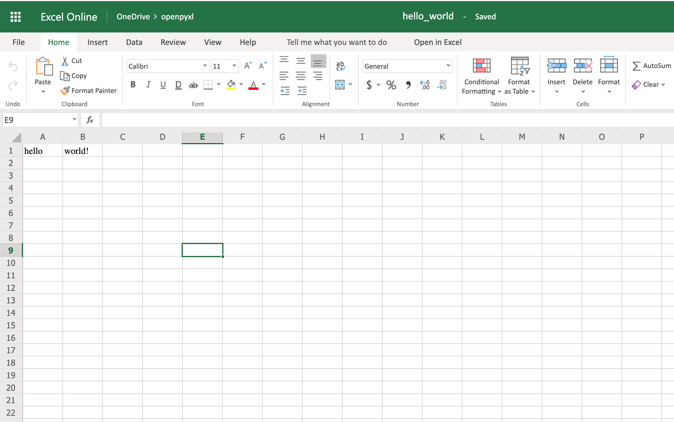
The code above should create a file called hello_world.xlsx in the folder you are using to run the code. If you open that file with Excel you should see something like this:

A Simple Hello World Spreadsheet

Woohoo, your first spreadsheet created!

Reading Excel Spreadsheets With openpyxl

Let’s start with the most essential thing one can do with a spreadsheet: read it.

You’ll go from a straightforward approach to reading a spreadsheet to more complex examples where you read the data and convert it into more useful Python structures.

Dataset for This Tutorial

Before you dive deep into some code examples, you should download this sample dataset and store it somewhere as sample.xlsx:

This is one of the datasets you’ll be using throughout this tutorial, and it’s a spreadsheet with a sample of real data from Amazon’s online product reviews. This dataset is only a tiny fraction of what Amazon provides, but for testing purposes, it’s more than enough.

A Simple Approach to Reading an Excel Spreadsheet

Finally, let’s start reading some spreadsheets! To begin with, open our sample spreadsheet:

>>>
>>> fromopenpyxlimportload_workbook>>> workbook=load_workbook(filename="sample.xlsx")>>> workbook.sheetnames['Sheet 1']>>> sheet=workbook.active>>> sheet<Worksheet "Sheet 1">>>> sheet.title'Sheet 1'

In the code above, you first open the spreadsheet sample.xlsx using load_workbook(), and then you can use workbook.sheetnames to see all the sheets you have available to work with. After that, workbook.active selects the first available sheet and, in this case, you can see that it selects Sheet 1 automatically. Using these methods is the default way of opening a spreadsheet, and you’ll see it many times during this tutorial.

Now, after opening a spreadsheet, you can easily retrieve data from it like this:

>>>
>>> sheet["A1"]<Cell 'Sheet 1'.A1>>>> sheet["A1"].value'marketplace'>>> sheet["F10"].value"G-Shock Men's Grey Sport Watch"

To return the actual value of a cell, you need to do .value. Otherwise, you’ll get the main Cell object. You can also use the method .cell() to retrieve a cell using index notation. Remember to add .value to get the actual value and not a Cell object:

>>>
>>> sheet.cell(row=10,column=6)<Cell 'Sheet 1'.F10>>>> sheet.cell(row=10,column=6).value"G-Shock Men's Grey Sport Watch"

You can see that the results returned are the same, no matter which way you decide to go with. However, in this tutorial, you’ll be mostly using the first approach: ["A1"].

Note: Even though in Python you’re used to a zero-indexed notation, with spreadsheets you’ll always use a one-indexed notation where the first row or column always has index 1.

The above shows you the quickest way to open a spreadsheet. However, you can pass additional parameters to change the way a spreadsheet is loaded.

Additional Reading Options

There are a few arguments you can pass to load_workbook() that change the way a spreadsheet is loaded. The most important ones are the following two Booleans:

  1. read_only loads a spreadsheet in read-only mode allowing you to open very large Excel files.
  2. data_only ignores loading formulas and instead loads only the resulting values.

Importing Data From a Spreadsheet

Now that you’ve learned the basics about loading a spreadsheet, it’s about time you get to the fun part: the iteration and actual usage of the values within the spreadsheet.

This section is where you’ll learn all the different ways you can iterate through the data, but also how to convert that data into something usable and, more importantly, how to do it in a Pythonic way.

Iterating Through the Data

There are a few different ways you can iterate through the data depending on your needs.

You can slice the data with a combination of columns and rows:

>>>
>>> sheet["A1:C2"]((<Cell 'Sheet 1'.A1>, <Cell 'Sheet 1'.B1>, <Cell 'Sheet 1'.C1>), (<Cell 'Sheet 1'.A2>, <Cell 'Sheet 1'.B2>, <Cell 'Sheet 1'.C2>))

You can get ranges of rows or columns:

>>>
>>> # Get all cells from column A>>> sheet["A"](<Cell 'Sheet 1'.A1>,<Cell 'Sheet 1'.A2>, ...<Cell 'Sheet 1'.A99>,<Cell 'Sheet 1'.A100>)>>> # Get all cells for a range of columns>>> sheet["A:B"]((<Cell 'Sheet 1'.A1>,<Cell 'Sheet 1'.A2>,  ...<Cell 'Sheet 1'.A99>,<Cell 'Sheet 1'.A100>), (<Cell 'Sheet 1'.B1>,<Cell 'Sheet 1'.B2>,  ...<Cell 'Sheet 1'.B99>,<Cell 'Sheet 1'.B100>))>>> # Get all cells from row 5>>> sheet[5](<Cell 'Sheet 1'.A5>,<Cell 'Sheet 1'.B5>, ...<Cell 'Sheet 1'.N5>,<Cell 'Sheet 1'.O5>)>>> # Get all cells for a range of rows>>> sheet[5:6]((<Cell 'Sheet 1'.A5>,<Cell 'Sheet 1'.B5>,  ...<Cell 'Sheet 1'.N5>,<Cell 'Sheet 1'.O5>), (<Cell 'Sheet 1'.A6>,<Cell 'Sheet 1'.B6>,  ...<Cell 'Sheet 1'.N6>,<Cell 'Sheet 1'.O6>))

You’ll notice that all of the above examples return a tuple. If you want to refresh your memory on how to handle tuples in Python, check out the article on Lists and Tuples in Python.

There are also multiple ways of using normal Python generators to go through the data. The main methods you can use to achieve this are:

  • .iter_rows()
  • .iter_cols()

Both methods can receive the following arguments:

  • min_row
  • max_row
  • min_col
  • max_col

These arguments are used to set boundaries for the iteration:

>>>
>>> forrowinsheet.iter_rows(min_row=1,... max_row=2,... min_col=1,... max_col=3):... print(row)(<Cell 'Sheet 1'.A1>, <Cell 'Sheet 1'.B1>, <Cell 'Sheet 1'.C1>)(<Cell 'Sheet 1'.A2>, <Cell 'Sheet 1'.B2>, <Cell 'Sheet 1'.C2>)>>> forcolumninsheet.iter_cols(min_row=1,... max_row=2,... min_col=1,... max_col=3):... print(column)(<Cell 'Sheet 1'.A1>, <Cell 'Sheet 1'.A2>)(<Cell 'Sheet 1'.B1>, <Cell 'Sheet 1'.B2>)(<Cell 'Sheet 1'.C1>, <Cell 'Sheet 1'.C2>)

You’ll notice that in the first example, when iterating through the rows using .iter_rows(), you get one tuple element per row selected. While when using .iter_cols() and iterating through columns, you’ll get one tuple per column instead.

One additional argument you can pass to both methods is the Boolean values_only. When it’s set to True, the values of the cell are returned, instead of the Cell object:

>>>
>>> forvalueinsheet.iter_rows(min_row=1,... max_row=2,... min_col=1,... max_col=3,... values_only=True):... print(value)('marketplace', 'customer_id', 'review_id')('US', 3653882, 'R3O9SGZBVQBV76')

If you want to iterate through the whole dataset, then you can also use the attributes .rows or .columns directly, which are shortcuts to using .iter_rows() and .iter_cols() without any arguments:

>>>
>>> forrowinsheet.rows:... print(row)(<Cell 'Sheet 1'.A1>, <Cell 'Sheet 1'.B1>, <Cell 'Sheet 1'.C1>...<Cell 'Sheet 1'.M100>, <Cell 'Sheet 1'.N100>, <Cell 'Sheet 1'.O100>)

These shortcuts are very useful when you’re iterating through the whole dataset.

Manipulate Data Using Python’s Default Data Structures

Now that you know the basics of iterating through the data in a workbook, let’s look at smart ways of converting that data into Python structures.

As you saw earlier, the result from all iterations comes in the form of tuples. However, since a tuple is nothing more than an immutable list, you can easily access its data and transform it into other structures.

For example, say you want to extract product information from the sample.xlsx spreadsheet and into a dictionary where each key is a product ID.

A straightforward way to do this is to iterate over all the rows, pick the columns you know are related to product information, and then store that in a dictionary. Let’s code this out!

First of all, have a look at the headers and see what information you care most about:

>>>
>>> forvalueinsheet.iter_rows(min_row=1,... max_row=1,... values_only=True):... print(value)('marketplace', 'customer_id', 'review_id', 'product_id', ...)

This code returns a list of all the column names you have in the spreadsheet. To start, grab the columns with names:

  • product_id
  • product_parent
  • product_title
  • product_category

Lucky for you, the columns you need are all next to each other so you can use the min_column and max_column to easily get the data you want:

>>>
>>> forvalueinsheet.iter_rows(min_row=2,... min_col=4,... max_col=7,... values_only=True):... print(value)('B00FALQ1ZC', 937001370, 'Invicta Women\'s 15150 "Angel" 18k Yellow...)('B00D3RGO20', 484010722, "Kenneth Cole New York Women's KC4944...)...

Nice! Now that you know how to get all the important product information you need, let’s put that data into a dictionary:

importjsonfromopenpyxlimportload_workbookworkbook=load_workbook(filename="sample.xlsx")sheet=workbook.activeproducts={}# Using the values_only because you want to return the cells' valuesforrowinsheet.iter_rows(min_row=2,min_col=4,max_col=7,values_only=True):product_id=row[0]product={"parent":row[1],"title":row[2],"category":row[3]}products[product_id]=product# Using json here to be able to format the output for displaying laterprint(json.dumps(products))

The code above returns a JSON similar to this:

{"B00FALQ1ZC":{"parent":937001370,"title":"Invicta Women's 15150 ...","category":"Watches"},"B00D3RGO20":{"parent":484010722,"title":"Kenneth Cole New York ...","category":"Watches"}}

Here you can see that the output is trimmed to 2 products only, but if you run the script as it is, then you should get 98 products.

Convert Data Into Python Classes

To finalize the reading section of this tutorial, let’s dive into Python classes and see how you could improve on the example above and better structure the data.

For this, you’ll be using the new Python Data Classes that are available from Python 3.7. If you’re using an older version of Python, then you can use the default Classes instead.

So, first things first, let’s look at the data you have and decide what you want to store and how you want to store it.

As you saw right at the start, this data comes from Amazon, and it’s a list of product reviews. You can check the list of all the columns and their meaning on Amazon.

There are two significant elements you can extract from the data available:

  1. Products
  2. Reviews

A Product has:

  • ID
  • Title
  • Parent
  • Category

The Review has a few more fields:

  • ID
  • Customer ID
  • Stars
  • Headline
  • Body
  • Date

You can ignore a few of the review fields to make things a bit simpler.

So, a straightforward implementation of these two classes could be written in a separate file classes.py:

importdatetimefromdataclassesimportdataclass@dataclassclassProduct:id:strparent:strtitle:strcategory:str@dataclassclassReview:id:strcustomer_id:strstars:intheadline:strbody:strdate:datetime.datetime

After defining your data classes, you need to convert the data from the spreadsheet into these new structures.

Before doing the conversion, it’s worth looking at our header again and creating a mapping between columns and the fields you need:

>>>
>>> forvalueinsheet.iter_rows(min_row=1,... max_row=1,... values_only=True):... print(value)('marketplace', 'customer_id', 'review_id', 'product_id', ...)>>> # Or an alternative>>> forcellinsheet[1]:... print(cell.value)marketplacecustomer_idreview_idproduct_idproduct_parent...

Let’s create a file mapping.py where you have a list of all the field names and their column location (zero-indexed) on the spreadsheet:

# Product fieldsPRODUCT_ID=3PRODUCT_PARENT=4PRODUCT_TITLE=5PRODUCT_CATEGORY=6# Review fieldsREVIEW_ID=2REVIEW_CUSTOMER=1REVIEW_STARS=7REVIEW_HEADLINE=12REVIEW_BODY=13REVIEW_DATE=14

You don’t necessarily have to do the mapping above. It’s more for readability when parsing the row data, so you don’t end up with a lot of magic numbers lying around.

Finally, let’s look at the code needed to parse the spreadsheet data into a list of product and review objects:

fromdatetimeimportdatetimefromopenpyxlimportload_workbookfromclassesimportProduct,ReviewfrommappingimportPRODUCT_ID,PRODUCT_PARENT,PRODUCT_TITLE, \
    PRODUCT_CATEGORY,REVIEW_DATE,REVIEW_ID,REVIEW_CUSTOMER, \
    REVIEW_STARS,REVIEW_HEADLINE,REVIEW_BODY# Using the read_only method since you're not gonna be editing the spreadsheetworkbook=load_workbook(filename="sample.xlsx",read_only=True)sheet=workbook.activeproducts=[]reviews=[]# Using the values_only because you just want to return the cell valueforrowinsheet.iter_rows(min_row=2,values_only=True):product=Product(id=row[PRODUCT_ID],parent=row[PRODUCT_PARENT],title=row[PRODUCT_TITLE],category=row[PRODUCT_CATEGORY])products.append(product)# You need to parse the date from the spreadsheet into a datetime formatspread_date=row[REVIEW_DATE]parsed_date=datetime.strptime(spread_date,"%Y-%m-%d")review=Review(id=row[REVIEW_ID],customer_id=row[REVIEW_CUSTOMER],stars=row[REVIEW_STARS],headline=row[REVIEW_HEADLINE],body=row[REVIEW_BODY],date=parsed_date)reviews.append(review)print(products[0])print(reviews[0])

After you run the code above, you should get some output like this:

Product(id='B00FALQ1ZC',parent=937001370,...)Review(id='R3O9SGZBVQBV76',customer_id=3653882,...)

That’s it! Now you should have the data in a very simple and digestible class format, and you can start thinking of storing this in a Database or any other type of data storage you like.

Using this kind of OOP strategy to parse spreadsheets makes handling the data much simpler later on.

Appending New Data

Before you start creating very complex spreadsheets, have a quick look at an example of how to append data to an existing spreadsheet.

Go back to the first example spreadsheet you created (hello_world.xlsx) and try opening it and appending some data to it, like this:

fromopenpyxlimportload_workbook# Start by opening the spreadsheet and selecting the main sheetworkbook=load_workbook(filename="hello_world.xlsx")sheet=workbook.active# Write what you want into a specific cellsheet["C1"]="writing ;)"# Save the spreadsheetworkbook.save(filename="hello_world_append.xlsx"

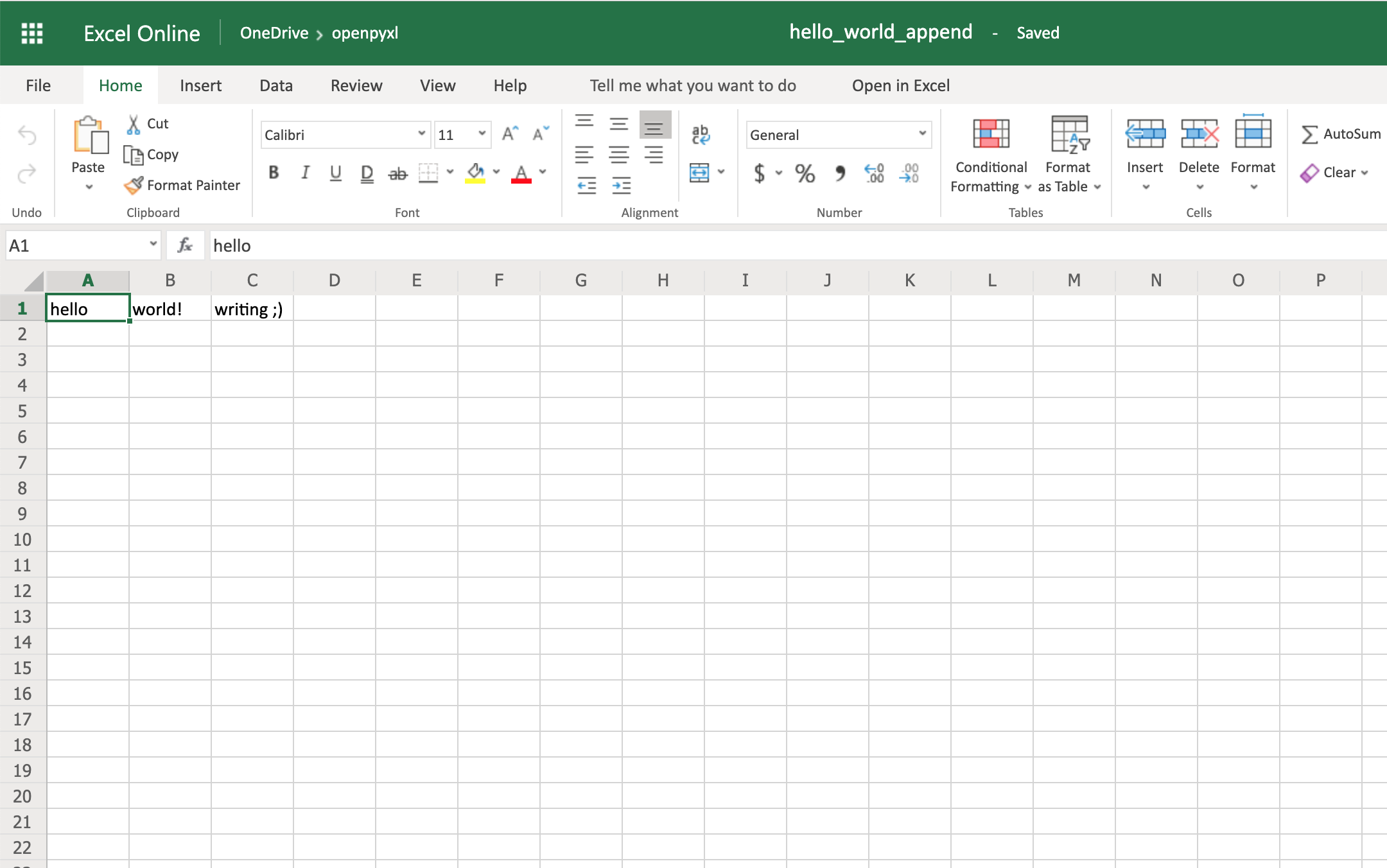
Et voilà, if you open the new hello_world_append.xlsx spreadsheet, you’ll see the following change:

Appending Data to a Spreadsheet

Notice the additional writing ;) on cell C1.

Writing Excel Spreadsheets With openpyxl

There are a lot of different things you can write to a spreadsheet, from simple text or number values to complex formulas, charts, or even images.

Let’s start creating some spreadsheets!

Creating a Simple Spreadsheet

Previously, you saw a very quick example of how to write “Hello world!” into a spreadsheet, so you can start with that:

 1 fromopenpyxlimportWorkbook 2  3 filename="hello_world.xlsx" 4  5 workbook=Workbook() 6 sheet=workbook.active 7  8 sheet["A1"]="hello" 9 sheet["B1"]="world!"10 11 workbook.save(filename=filename)

The highlighted lines in the code above are the most important ones for writing. In the code, you can see that:

  • Line 5 shows you how to create a new empty workbook.
  • Lines 8 and 9 show you how to add data to specific cells.
  • Line 11 shows you how to save the spreadsheet when you’re done.

Even though these lines above can be straightforward, it’s still good to know them well for when things get a bit more complicated.

Note: You’ll be using the hello_world.xlsx spreadsheet for some of the upcoming examples, so keep it handy.

One thing you can do to help with coming code examples is add the following method to your Python file or console:

>>>
>>> defprint_rows():... forrowinsheet.iter_rows(values_only=True):... print(row)

It makes it easier to print all of your spreadsheet values by just calling print_rows().

Basic Spreadsheet Operations

Before you get into the more advanced topics, it’s good for you to know how to manage the most simple elements of a spreadsheet.

Adding and Updating Cell Values

You already learned how to add values to a spreadsheet like this:

>>>
>>> sheet["A1"]="value"

There’s another way you can do this, by first selecting a cell and then changing its value:

>>>
>>> cell=sheet["A1"]>>> cell<Cell 'Sheet'.A1>>>> cell.value'hello'>>> cell.value="hey">>> cell.value'hey'

The new value is only stored into the spreadsheet once you call workbook.save().

The openpyxl creates a cell when adding a value, if that cell didn’t exist before:

>>>
>>> # Before, our spreadsheet has only 1 row>>> print_rows()('hello', 'world!')>>> # Try adding a value to row 10>>> sheet["B10"]="test">>> print_rows()('hello', 'world!')(None, None)(None, None)(None, None)(None, None)(None, None)(None, None)(None, None)(None, None)(None, 'test')

As you can see, when trying to add a value to cell B10, you end up with a tuple with 10 rows, just so you can have that test value.

Managing Rows and Columns

One of the most common things you have to do when manipulating spreadsheets is adding or removing rows and columns. The openpyxl package allows you to do that in a very straightforward way by using the methods:

  • .insert_rows()
  • .delete_rows()
  • .insert_cols()
  • .delete_cols()

Every single one of those methods can receive two arguments:

  1. idx
  2. amount

Using our basic hello_world.xlsx example again, let’s see how these methods work:

>>>
>>> print_rows()('hello', 'world!')>>> # Insert a column before the existing column 1 ("A")>>> sheet.insert_cols(idx=1)>>> print_rows()(None, 'hello', 'world!')>>> # Insert 5 columns between column 2 ("B") and 3 ("C")>>> sheet.insert_cols(idx=3,amount=5)>>> print_rows()(None, 'hello', None, None, None, None, None, 'world!')>>> # Delete the created columns>>> sheet.delete_cols(idx=3,amount=5)>>> sheet.delete_cols(idx=1)>>> print_rows()('hello', 'world!')>>> # Insert a new row in the beginning>>> sheet.insert_rows(idx=1)>>> print_rows()(None, None)('hello', 'world!')>>> # Insert 3 new rows in the beginning>>> sheet.insert_rows(idx=1,amount=3)>>> print_rows()(None, None)(None, None)(None, None)(None, None)('hello', 'world!')>>> # Delete the first 4 rows>>> sheet.delete_rows(idx=1,amount=4)>>> print_rows()('hello', 'world!')

The only thing you need to remember is that when inserting new data (rows or columns), the insertion happens before the idx parameter.

So, if you do insert_rows(1), it inserts a new row before the existing first row.

It’s the same for columns: when you call insert_cols(2), it inserts a new column right before the already existing second column (B).

However, when deleting rows or columns, .delete_... deletes data starting from the index passed as an argument.

For example, when doing delete_rows(2) it deletes row 2, and when doing delete_cols(3) it deletes the third column (C).

Managing Sheets

Sheet management is also one of those things you might need to know, even though it might be something that you don’t use that often.

If you look back at the code examples from this tutorial, you’ll notice the following recurring piece of code:

sheet=workbook.active

This is the way to select the default sheet from a spreadsheet. However, if you’re opening a spreadsheet with multiple sheets, then you can always select a specific one like this:

>>>
>>> # Let's say you have two sheets: "Products" and "Company Sales">>> workbook.sheetnames['Products', 'Company Sales']>>> # You can select a sheet using its title>>> products_sheet=workbook["Products"]>>> sales_sheet=workbook["Company Sales"]

You can also change a sheet title very easily:

>>>
>>> workbook.sheetnames['Products', 'Company Sales']>>> products_sheet=workbook["Products"]>>> products_sheet.title="New Products">>> workbook.sheetnames['New Products', 'Company Sales']

If you want to create or delete sheets, then you can also do that with .create_sheet() and .remove():

>>>
>>> workbook.sheetnames['Products', 'Company Sales']>>> operations_sheet=workbook.create_sheet("Operations")>>> workbook.sheetnames['Products', 'Company Sales', 'Operations']>>> # You can also define the position to create the sheet at>>> hr_sheet=workbook.create_sheet("HR",0)>>> workbook.sheetnames['HR', 'Products', 'Company Sales', 'Operations']>>> # To remove them, just pass the sheet as an argument to the .remove()>>> workbook.remove(operations_sheet)>>> workbook.sheetnames['HR', 'Products', 'Company Sales']>>> workbook.remove(hr_sheet)>>> workbook.sheetnames['Products', 'Company Sales']

One other thing you can do is make duplicates of a sheet using copy_worksheet():

>>>
>>> workbook.sheetnames['Products', 'Company Sales']>>> products_sheet=workbook["Products"]>>> workbook.copy_worksheet(products_sheet)<Worksheet "Products Copy">>>> workbook.sheetnames['Products', 'Company Sales', 'Products Copy']

If you open your spreadsheet after saving the above code, you’ll notice that the sheet Products Copy is a duplicate of the sheet Products.

Freezing Rows and Columns

Something that you might want to do when working with big spreadsheets is to freeze a few rows or columns, so they remain visible when you scroll right or down.

Freezing data allows you to keep an eye on important rows or columns, regardless of where you scroll in the spreadsheet.

Again, openpyxl also has a way to accomplish this by using the worksheet freeze_panes attribute. For this example, go back to our sample.xlsx spreadsheet and try doing the following:

>>>
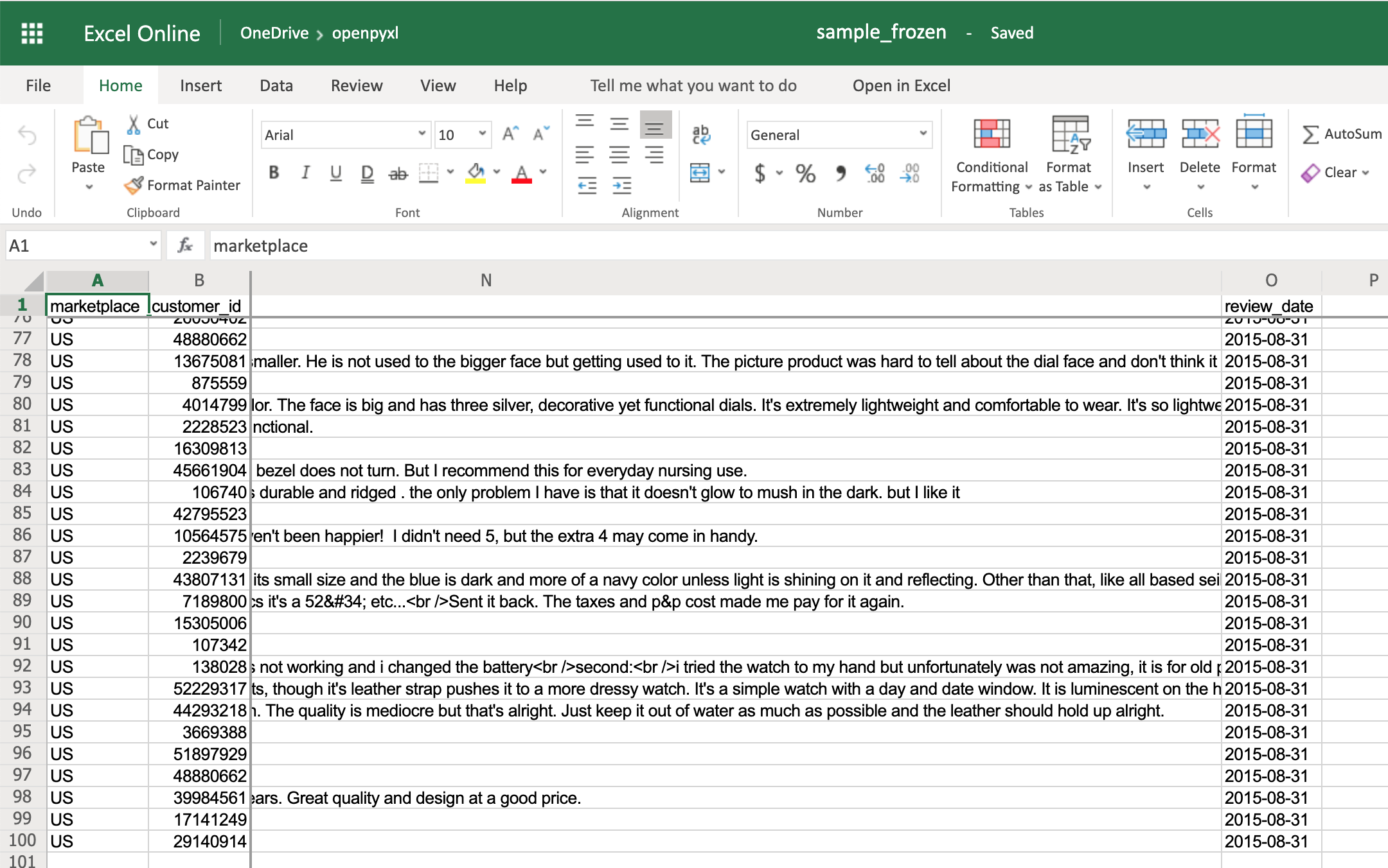
>>> workbook=load_workbook(filename="sample.xlsx")>>> sheet=workbook.active>>> sheet.freeze_panes="C2">>> workbook.save("sample_frozen.xlsx")

If you open the sample_frozen.xlsx spreadsheet in your favorite spreadsheet editor, you’ll notice that row 1 and columns A and B are frozen and are always visible no matter where you navigate within the spreadsheet.

This feature is handy, for example, to keep headers within sight, so you always know what each column represents.

Here’s how it looks in the editor:

Example Spreadsheet With Frozen Rows and Columns

Notice how you’re at the end of the spreadsheet, and yet, you can see both row 1 and columns A and B.

Adding Filters

You can use openpyxl to add filters and sorts to your spreadsheet. However, when you open the spreadsheet, the data won’t be rearranged according to these sorts and filters.

At first, this might seem like a pretty useless feature, but when you’re programmatically creating a spreadsheet that is going to be sent and used by somebody else, it’s still nice to at least create the filters and allow people to use it afterward.

The code below is an example of how you would add some filters to our existing sample.xlsx spreadsheet:

>>>
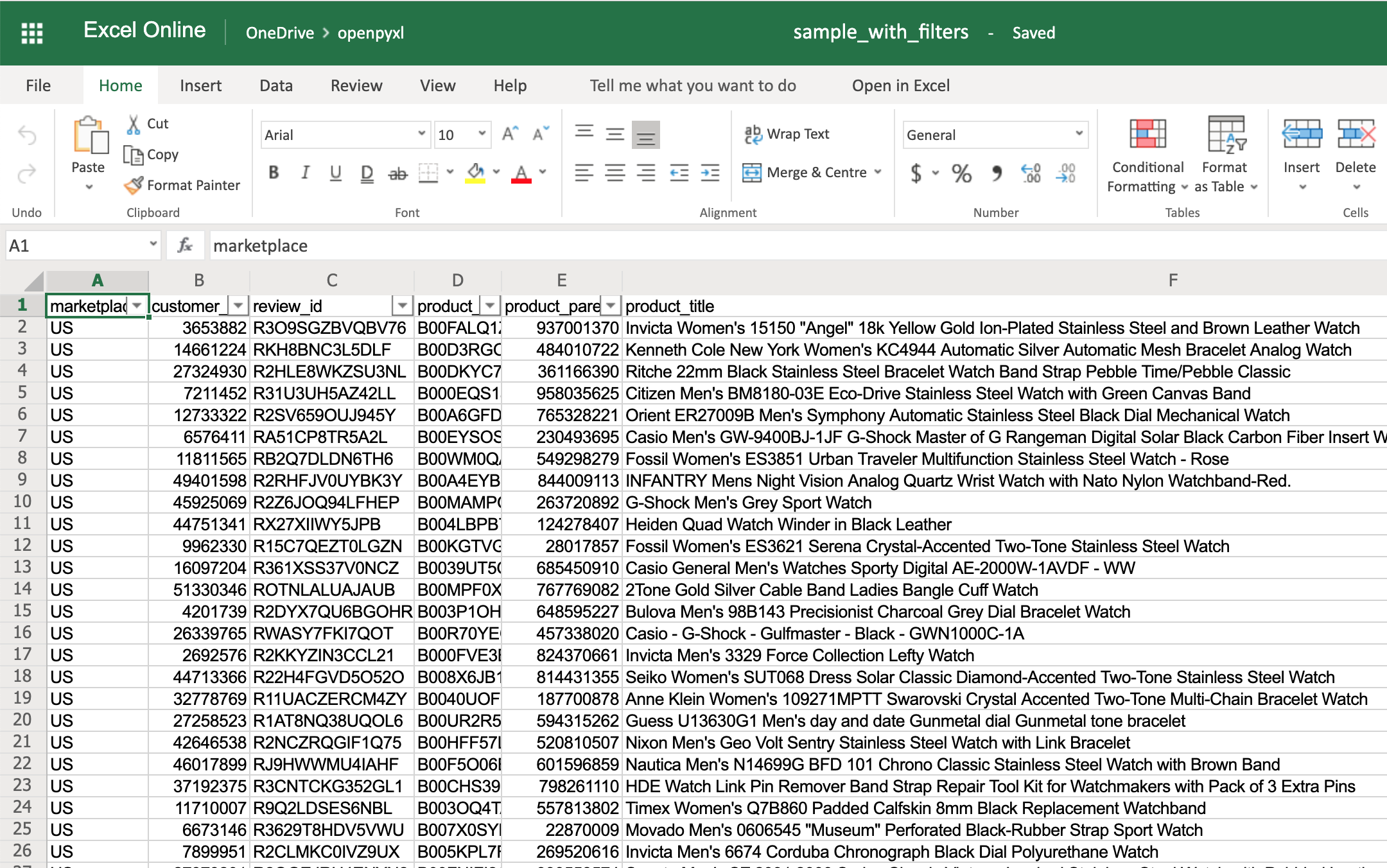
>>> # Check the used spreadsheet space using the attribute "dimensions">>> sheet.dimensions'A1:O100'>>> sheet.auto_filter.ref="A1:O100">>> workbook.save(filename="sample_with_filters.xlsx")

You should now see the filters created when opening the spreadsheet in your editor:

Example Spreadsheet With Filters

You don’t have to use sheet.dimensions if you know precisely which part of the spreadsheet you want to apply filters to.

Adding Formulas

Formulas (or formulae) are one of the most powerful features of spreadsheets.

They gives you the power to apply specific mathematical equations to a range of cells. Using formulas with openpyxl is as simple as editing the value of a cell.

You can see the list of formulas supported by openpyxl:

>>>
>>> fromopenpyxl.utilsimportFORMULAE>>> FORMULAEfrozenset({'ABS',           'ACCRINT',           'ACCRINTM',           'ACOS',           'ACOSH',           'AMORDEGRC',           'AMORLINC',           'AND',           ...           'YEARFRAC',           'YIELD',           'YIELDDISC',           'YIELDMAT',           'ZTEST'})

Let’s add some formulas to our sample.xlsx spreadsheet.

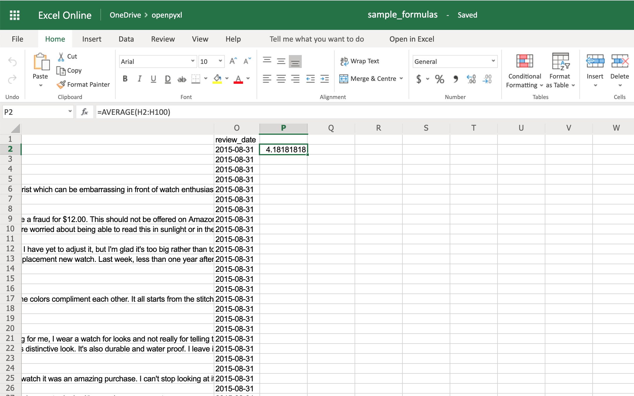
Starting with something easy, let’s check the average star rating for the 99 reviews within the spreadsheet:

>>>
>>> # Star rating is column "H">>> sheet["P2"]="=AVERAGE(H2:H100)">>> workbook.save(filename="sample_formulas.xlsx")

If you open the spreadsheet now and go to cell P2, you should see that its value is: 4.18181818181818. Have a look in the editor:

Example Spreadsheet With Average Formula

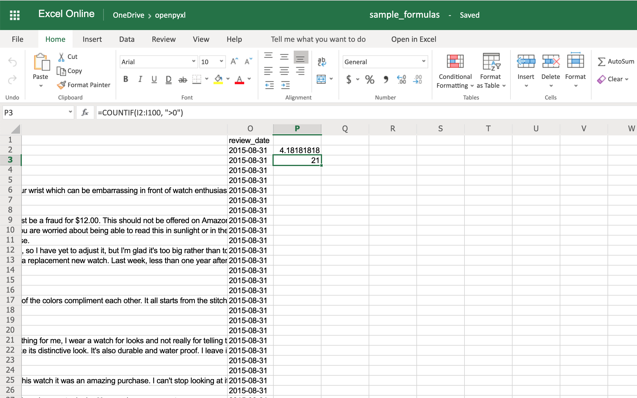
You can use the same methodology to add any formulas to your spreadsheet. For example, let’s count the number of reviews that had helpful votes:

>>>
>>> # The helpful votes are counted on column "I">>> sheet["P3"]='=COUNTIF(I2:I100, ">0")'>>> workbook.save(filename="sample_formulas.xlsx")

You should get the number 21 on your P3 spreadsheet cell like so:

Example Spreadsheet With Average and CountIf Formula

You’ll have to make sure that the strings within a formula are always in double quotes, so you either have to use single quotes around the formula like in the example above or you’ll have to escape the double quotes inside the formula: "=COUNTIF(I2:I100, \">0\")".

There are a ton of other formulas you can add to your spreadsheet using the same procedure you tried above. Give it a go yourself!

Adding Styles

Even though styling a spreadsheet might not be something you would do every day, it’s still good to know how to do it.

Using openpyxl, you can apply multiple styling options to your spreadsheet, including fonts, borders, colors, and so on. Have a look at the openpyxldocumentation to learn more.

You can also choose to either apply a style directly to a cell or create a template and reuse it to apply styles to multiple cells.

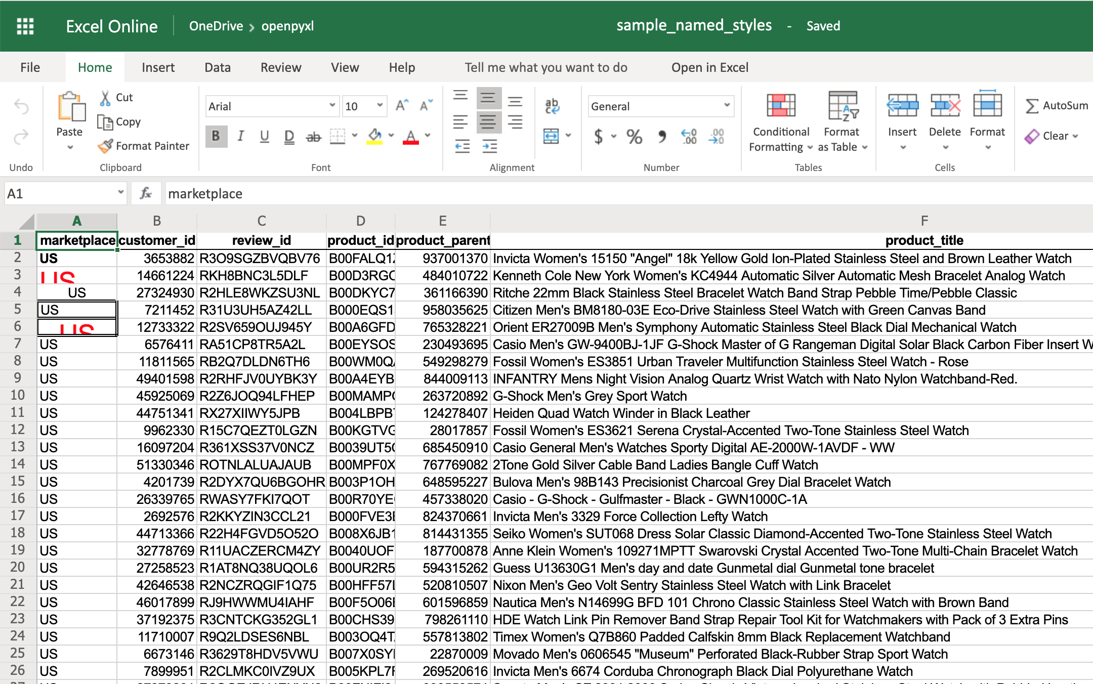
Let’s start by having a look at simple cell styling, using our sample.xlsx again as the base spreadsheet:

>>>
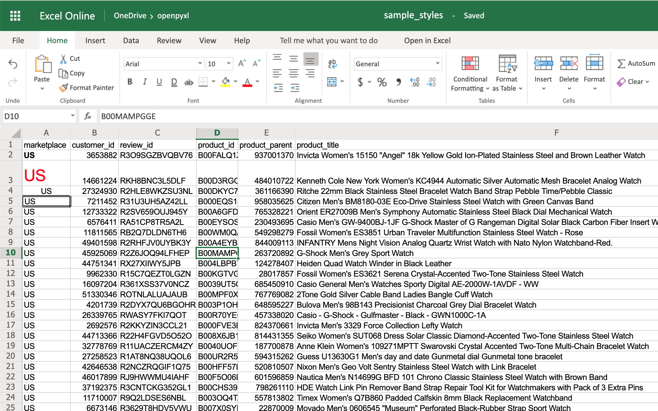
>>> # Import necessary style classes>>> fromopenpyxl.stylesimportFont,Color,Alignment,Border,Side,colors>>> # Create a few styles>>> bold_font=Font(bold=True)>>> big_red_text=Font(color=colors.RED,size=20)>>> center_aligned_text=Alignment(horizontal="center")>>> double_border_side=Side(border_style="double")>>> square_border=Border(top=double_border_side,... right=double_border_side,... bottom=double_border_side,... left=double_border_side)>>> # Style some cells!>>> sheet["A2"].font=bold_font>>> sheet["A3"].font=big_red_text>>> sheet["A4"].alignment=center_aligned_text>>> sheet["A5"].border=square_border>>> workbook.save(filename="sample_styles.xlsx")

If you open your spreadsheet now, you should see quite a few different styles on the first 5 cells of column A:

Example Spreadsheet With Simple Cell Styles

There you go. You got:

  • A2 with the text in bold
  • A3 with the text in red and bigger font size
  • A4 with the text centered
  • A5 with a square border around the text

Note: For the colors, you can also use HEX codes instead by doing Font(color="C70E0F").

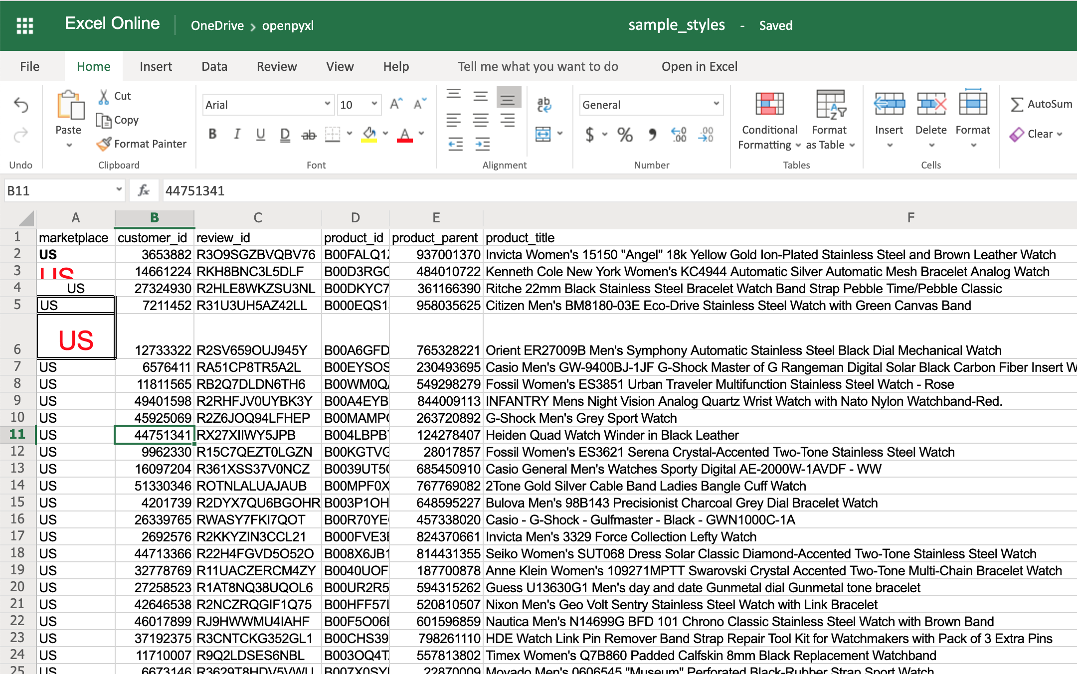
You can also combine styles by simply adding them to the cell at the same time:

>>>
>>> # Reusing the same styles from the example above>>> sheet["A6"].alignment=center_aligned_text>>> sheet["A6"].font=big_red_text>>> sheet["A6"].border=square_border>>> workbook.save(filename="sample_styles.xlsx")

Have a look at cell A6 here:

Example Spreadsheet With Coupled Cell Styles

When you want to apply multiple styles to one or several cells, you can use a NamedStyle class instead, which is like a style template that you can use over and over again. Have a look at the example below:

>>>
>>> fromopenpyxl.stylesimportNamedStyle>>> # Let's create a style template for the header row>>> header=NamedStyle(name="header")>>> header.font=Font(bold=True)>>> header.border=Border(bottom=Side(border_style="thin"))>>> header.alignment=Alignment(horizontal="center",vertical="center")>>> # Now let's apply this to all first row (header) cells>>> header_row=sheet[1]>>> forcellinheader_row:... cell.style=header>>> workbook.save(filename="sample_styles.xlsx")

If you open the spreadsheet now, you should see that its first row is bold, the text is aligned to the center, and there’s a small bottom border! Have a look below:

Example Spreadsheet With Named Styles

As you saw above, there are many options when it comes to styling, and it depends on the use case, so feel free to check openpyxldocumentation and see what other things you can do.

Conditional Formatting

This feature is one of my personal favorites when it comes to adding styles to a spreadsheet.

It’s a much more powerful approach to styling because it dynamically applies styles according to how the data in the spreadsheet changes.

In a nutshell, conditional formatting allows you to specify a list of styles to apply to a cell (or cell range) according to specific conditions.

For example, a widespread use case is to have a balance sheet where all the negative totals are in red, and the positive ones are in green. This formatting makes it much more efficient to spot good vs bad periods.

Without further ado, let’s pick our favorite spreadsheet—sample.xlsx—and add some conditional formatting.

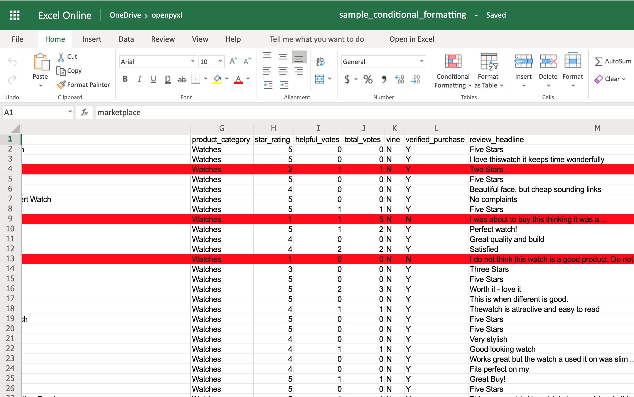
You can start by adding a simple one that adds a red background to all reviews with less than 3 stars:

>>>
>>> fromopenpyxl.stylesimportPatternFill,colors>>> fromopenpyxl.styles.differentialimportDifferentialStyle>>> fromopenpyxl.formatting.ruleimportRule>>> red_background=PatternFill(bgColor=colors.RED)>>> diff_style=DifferentialStyle(fill=red_background)>>> rule=Rule(type="expression",dxf=diff_style)>>> rule.formula=["$H1<3"]>>> sheet.conditional_formatting.add("A1:O100",rule)>>> workbook.save("sample_conditional_formatting.xlsx.xlsx")

Now you’ll see all the reviews with a star rating below 3 marked with a red background:

Example Spreadsheet With Simple Conditional Formatting

Code-wise, the only things that are new here are the objects DifferentialStyle and Rule:

  • DifferentialStyle is quite similar to NamedStyle, which you already saw above, and it’s used to aggregate multiple styles such as fonts, borders, alignment, and so forth.
  • Rule is responsible for selecting the cells and applying the styles if the cells match the rule’s logic.

Using a Rule object, you can create numerous conditional formatting scenarios.

However, for simplicity sake, the openpyxl package offers 3 built-in formats that make it easier to create a few common conditional formatting patterns. These built-ins are:

  • ColorScale
  • IconSet
  • DataBar

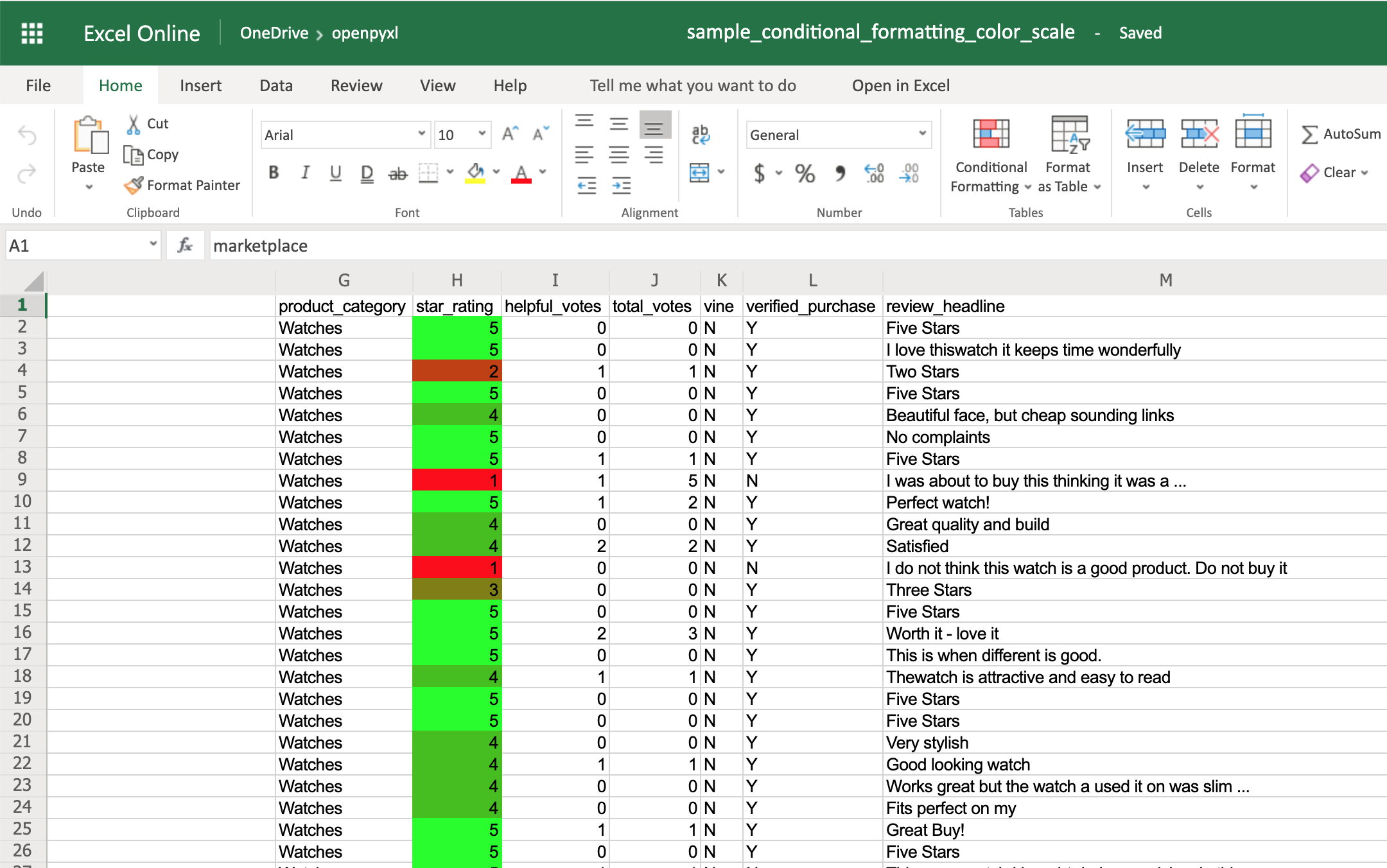
The ColorScale gives you the ability to create color gradients:

>>>
>>> fromopenpyxl.formatting.ruleimportColorScaleRule>>> color_scale_rule=ColorScaleRule(start_type="min",... start_color=colors.RED,... end_type="max",... end_color=colors.GREEN)>>> # Again, let's add this gradient to the star ratings, column "H">>> sheet.conditional_formatting.add("H2:H100",color_scale_rule)>>> workbook.save(filename="sample_conditional_formatting_color_scale.xlsx")

Now you should see a color gradient on column H, from red to green, according to the star rating:

Example Spreadsheet With Color Scale Conditional Formatting

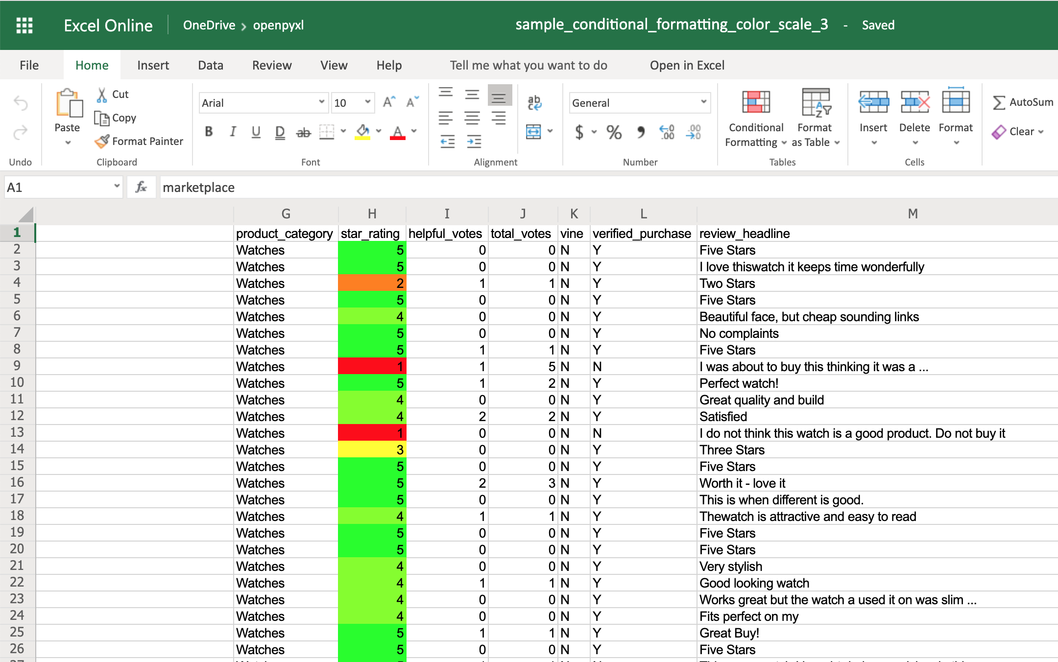
You can also add a third color and make two gradients instead:

>>>
>>> fromopenpyxl.formatting.ruleimportColorScaleRule>>> color_scale_rule=ColorScaleRule(start_type="num",... start_value=1,... start_color=colors.RED,... mid_type="num",... mid_value=3,... mid_color=colors.YELLOW,... end_type="num",... end_value=5,... end_color=colors.GREEN)>>> # Again, let's add this gradient to the star ratings, column "H">>> sheet.conditional_formatting.add("H2:H100",color_scale_rule)>>> workbook.save(filename="sample_conditional_formatting_color_scale_3.xlsx")

This time, you’ll notice that star ratings between 1 and 3 have a gradient from red to yellow, and star ratings between 3 and 5 have a gradient from yellow to green:

Example Spreadsheet With 2 Color Scales Conditional Formatting

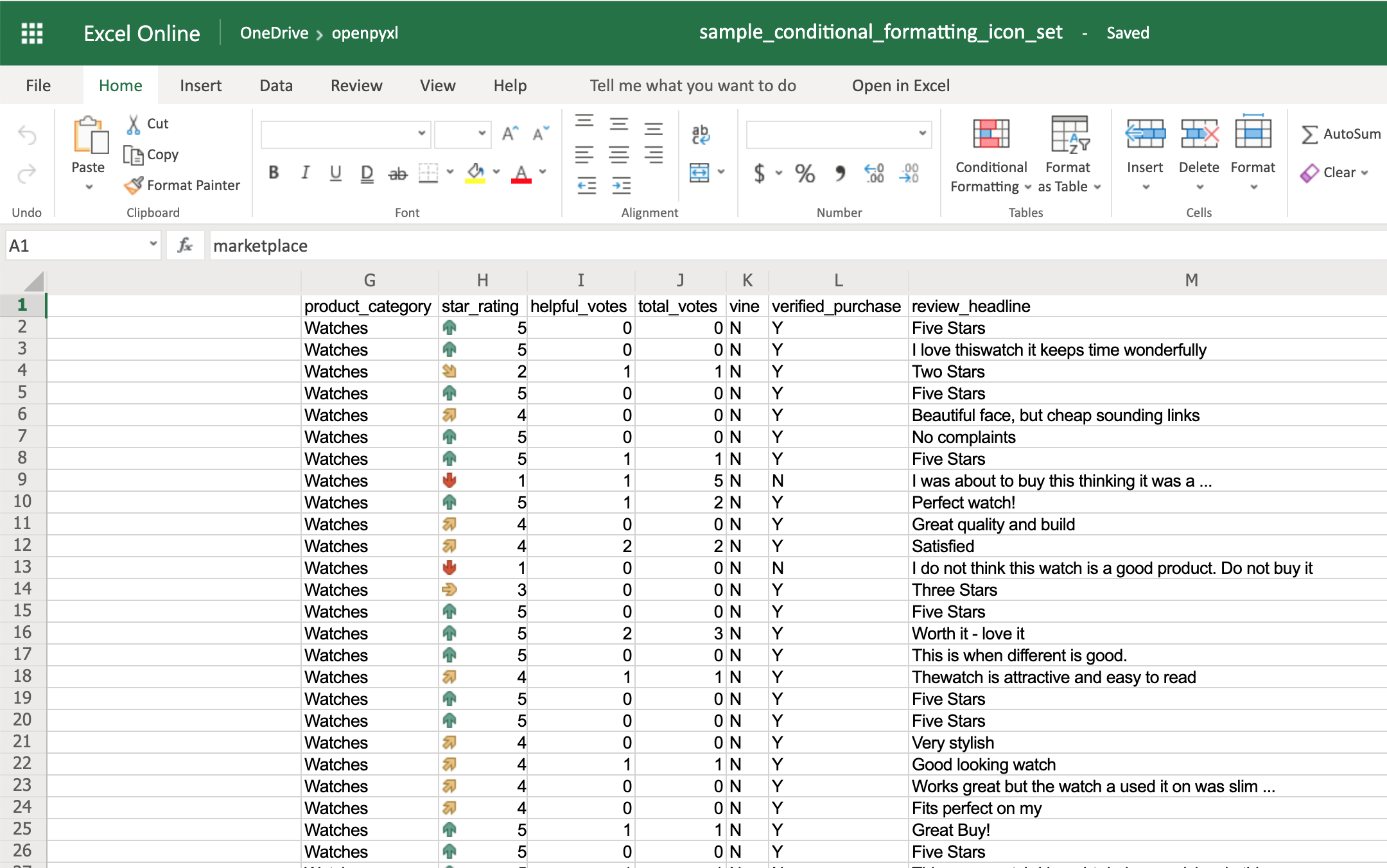
The IconSet allows you to add an icon to the cell according to its value:

>>>
>>> fromopenpyxl.formatting.ruleimportIconSetRule>>> icon_set_rule=IconSetRule("5Arrows","num",[1,2,3,4,5])>>> sheet.conditional_formatting.add("H2:H100",icon_set_rule)>>> workbook.save("sample_conditional_formatting_icon_set.xlsx")

You’ll see a colored arrow next to the star rating. This arrow is red and points down when the value of the cell is 1 and, as the rating gets better, the arrow starts pointing up and becomes green:

Example Spreadsheet With Icon Set Conditional Formatting

The openpyxl package has a full list of other icons you can use, besides the arrow.

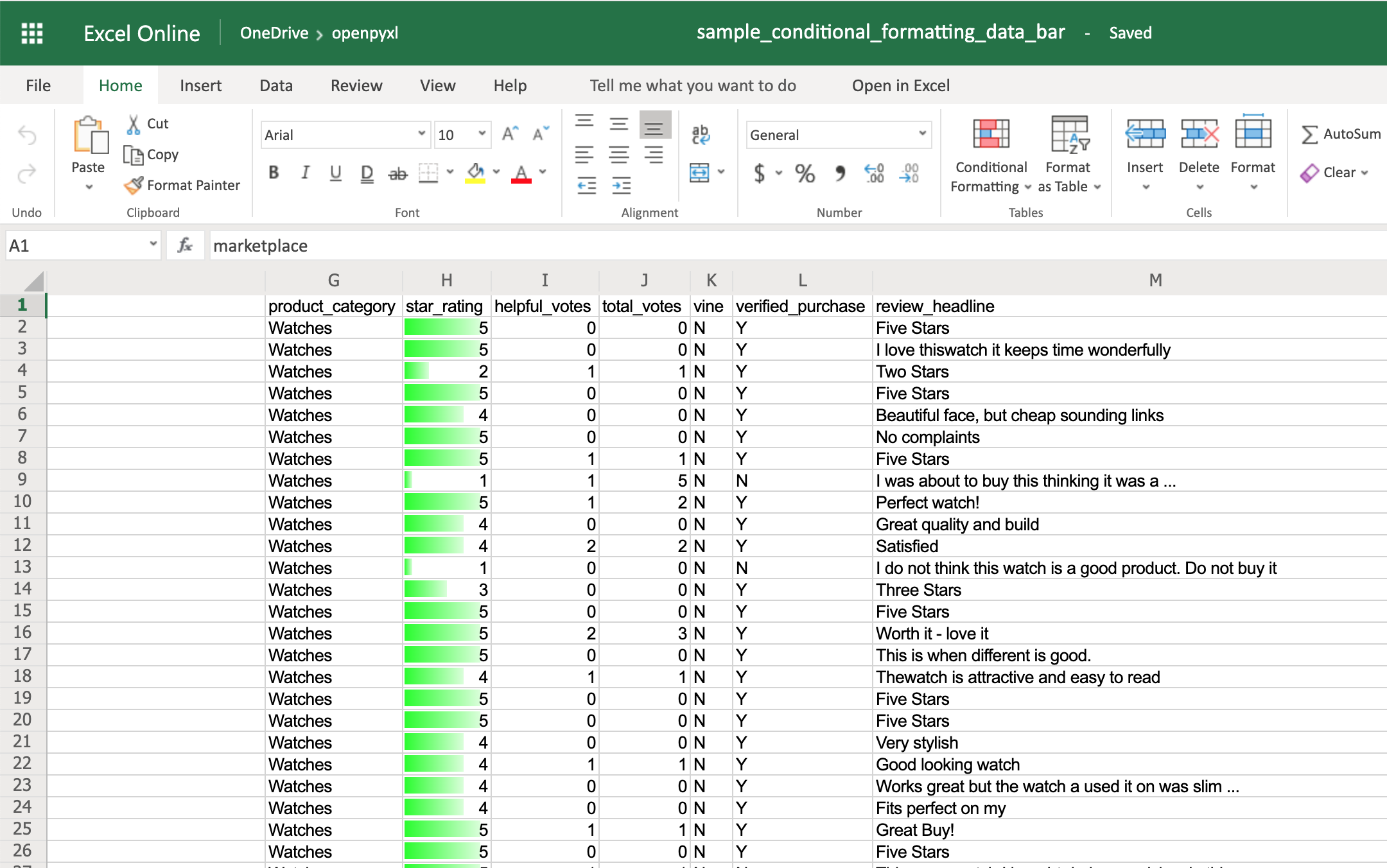
Finally, the DataBar allows you to create progress bars:

>>>
>>> fromopenpyxl.formatting.ruleimportDataBarRule>>> data_bar_rule=DataBarRule(start_type="num",... start_value=1,... end_type="num",... end_value="5",... color=colors.GREEN)>>> sheet.conditional_formatting.add("H2:H100",data_bar_rule)>>> workbook.save("sample_conditional_formatting_data_bar.xlsx")

You’ll now see a green progress bar that gets fuller the closer the star rating is to the number 5:

Example Spreadsheet With Data Bar Conditional Formatting

As you can see, there are a lot of cool things you can do with conditional formatting.

Here, you saw only a few examples of what you can achieve with it, but check the openpyxldocumentation to see a bunch of other options.

Adding Images

Even though images are not something that you’ll often see in a spreadsheet, it’s quite cool to be able to add them. Maybe you can use it for branding purposes or to make spreadsheets more personal.

To be able to load images to a spreadsheet using openpyxl, you’ll have to install Pillow:

$ pip install Pillow

Apart from that, you’ll also need an image. For this example, you can grab the Real Python logo below and convert it from .webp to .png using an online converter such as cloudconvert.com, save the final file as logo.png, and copy it to the root folder where you’re running your examples:

Real Python Logo

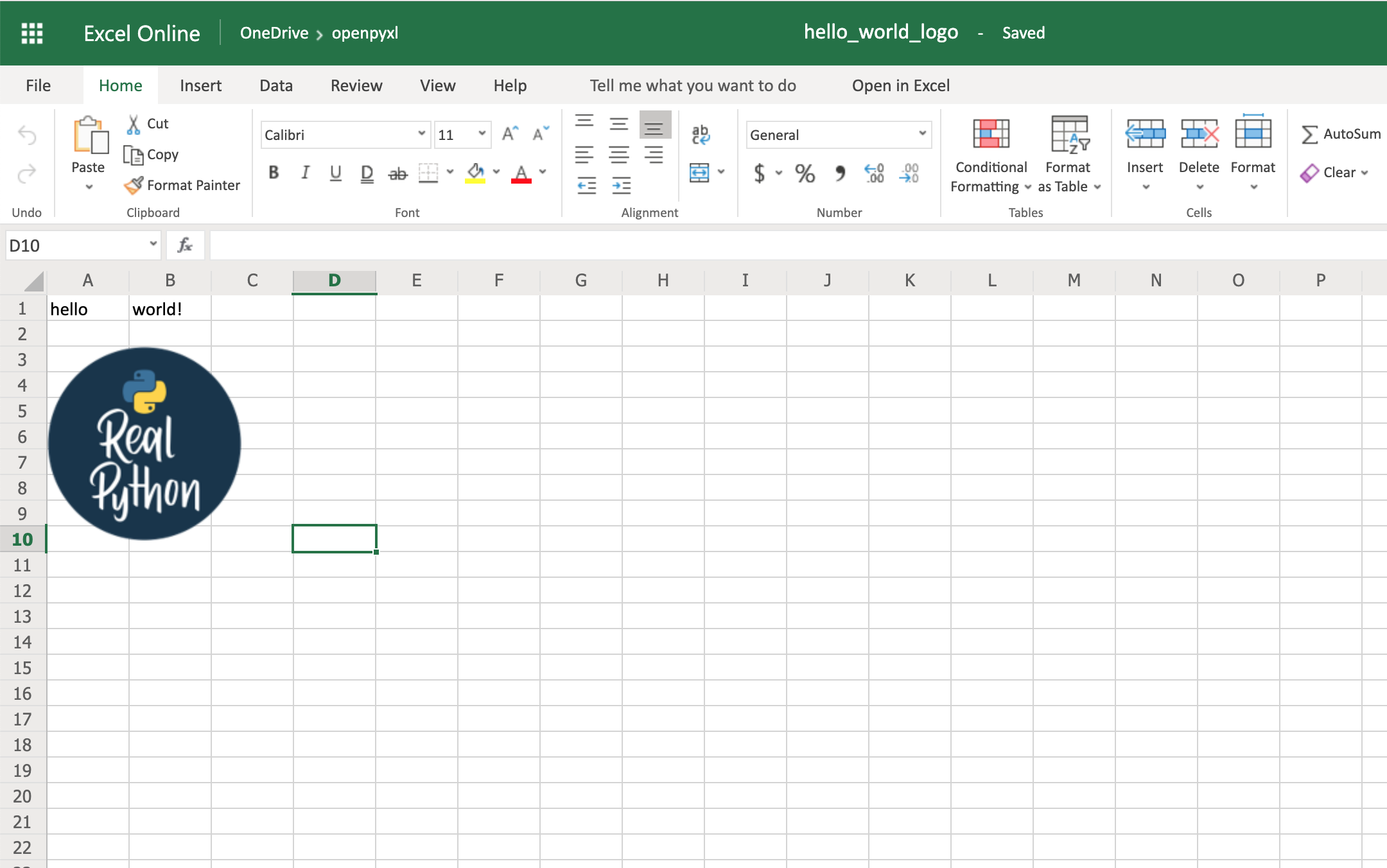
Afterward, this is the code you need to import that image into the hello_word.xlsx spreadsheet:

fromopenpyxlimportload_workbookfromopenpyxl.drawing.imageimportImage# Let's use the hello_world spreadsheet since it has less dataworkbook=load_workbook(filename="hello_world.xlsx")sheet=workbook.activelogo=Image("logo.png")# A bit of resizing to not fill the whole spreadsheet with the logologo.height=150logo.width=150sheet.add_image(logo,"A3")workbook.save(filename="hello_world_logo.xlsx")

You have an image on your spreadsheet! Here it is:

Example Spreadsheet With Image

The image’s left top corner is on the cell you chose, in this case, A3.

Adding Pretty Charts

Another powerful thing you can do with spreadsheets is create an incredible variety of charts.

Charts are a great way to visualize and understand loads of data quickly. There are a lot of different chart types: bar chart, pie chart, line chart, and so on. openpyxl has support for a lot of them.

Here, you’ll see only a couple of examples of charts because the theory behind it is the same for every single chart type:

Note: A few of the chart types that openpyxl currently doesn’t have support for are Funnel, Gantt, Pareto, Treemap, Waterfall, Map, and Sunburst.

For any chart you want to build, you’ll need to define the chart type: BarChart, LineChart, and so forth, plus the data to be used for the chart, which is called Reference.

Before you can build your chart, you need to define what data you want to see represented in it. Sometimes, you can use the dataset as is, but other times you need to massage the data a bit to get additional information.

Let’s start by building a new workbook with some sample data:

 1 fromopenpyxlimportWorkbook 2 fromopenpyxl.chartimportBarChart,Reference 3  4 workbook=Workbook() 5 sheet=workbook.active 6  7 # Let's create some sample sales data 8 rows=[ 9 ["Product","Online","Store"],10 [1,30,45],11 [2,40,30],12 [3,40,25],13 [4,50,30],14 [5,30,25],15 [6,25,35],16 [7,20,40],17 ]18 19 forrowinrows:20 sheet.append(row)

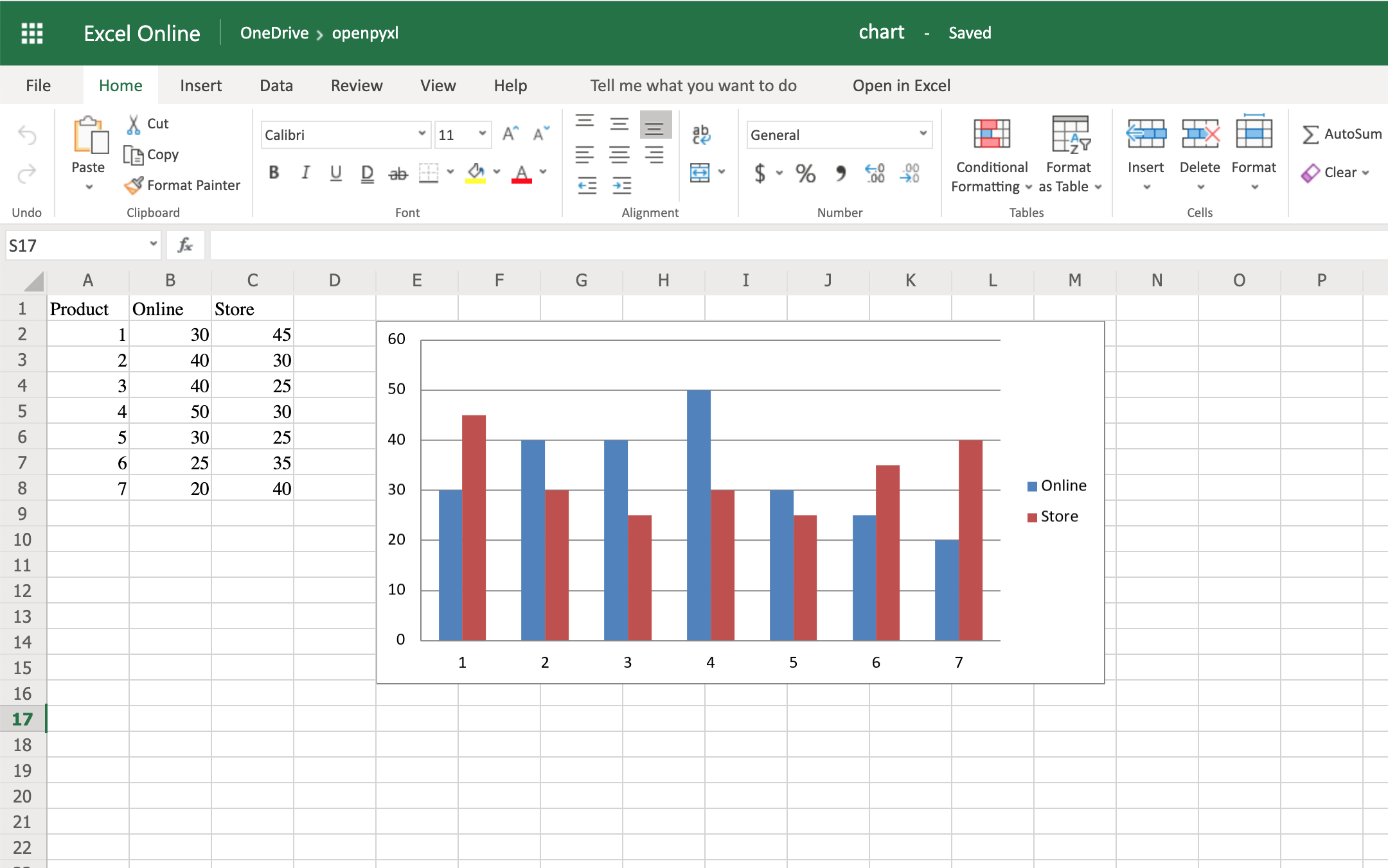
Now you’re going to start by creating a bar chart that displays the total number of sales per product:

22 chart=BarChart()23 data=Reference(worksheet=sheet,24 min_row=1,25 max_row=8,26 min_col=2,27 max_col=3)28 29 chart.add_data(data,titles_from_data=True)30 sheet.add_chart(chart,"E2")31 32 workbook.save("chart.xlsx")

There you have it. Below, you can see a very straightforward bar chart showing the difference between online product sales online and in-store product sales:

Example Spreadsheet With Bar Chart

Like with images, the top left corner of the chart is on the cell you added the chart to. In your case, it was on cell E2.

Note: Depending on whether you’re using Microsoft Excel or an open-source alternative (LibreOffice or OpenOffice), the chart might look slightly different.

Try creating a line chart instead, changing the data a bit:

 1 importrandom 2 fromopenpyxlimportWorkbook 3 fromopenpyxl.chartimportLineChart,Reference 4  5 workbook=Workbook() 6 sheet=workbook.active 7  8 # Let's create some sample sales data 9 rows=[10 ["","January","February","March","April",11 "May","June","July","August","September",12 "October","November","December"],13 [1,],14 [2,],15 [3,],16 ]17 18 forrowinrows:19 sheet.append(row)20 21 forrowinsheet.iter_rows(min_row=2,22 max_row=4,23 min_col=2,24 max_col=13):25 forcellinrow:26 cell.value=random.randrange(5,100)

With the above code, you’ll be able to generate some random data regarding the sales of 3 different products across a whole year.

Once that’s done, you can very easily create a line chart with the following code:

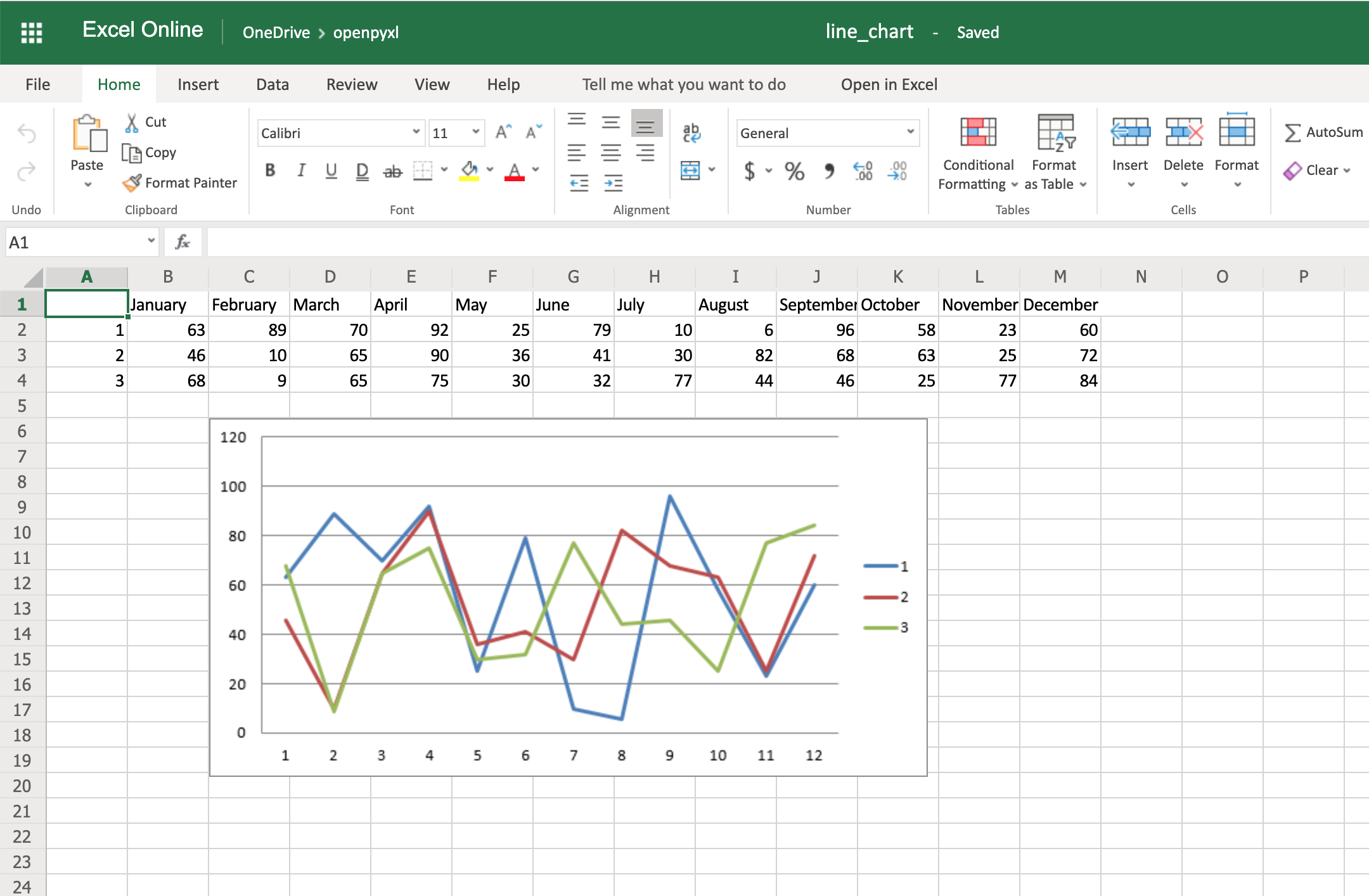
28 chart=LineChart()29 data=Reference(worksheet=sheet,30 min_row=2,31 max_row=4,32 min_col=1,33 max_col=13)34 35 chart.add_data(data,from_rows=True,titles_from_data=True)36 sheet.add_chart(chart,"C6")37 38 workbook.save("line_chart.xlsx")

Here’s the outcome of the above piece of code:

Example Spreadsheet With Line Chart

One thing to keep in mind here is the fact that you’re using from_rows=True when adding the data. This argument makes the chart plot row by row instead of column by column.

In your sample data, you see that each product has a row with 12 values (1 column per month). That’s why you use from_rows. If you don’t pass that argument, by default, the chart tries to plot by column, and you’ll get a month-by-month comparison of sales.

Another difference that has to do with the above argument change is the fact that our Reference now starts from the first column, min_col=1, instead of the second one. This change is needed because the chart now expects the first column to have the titles.

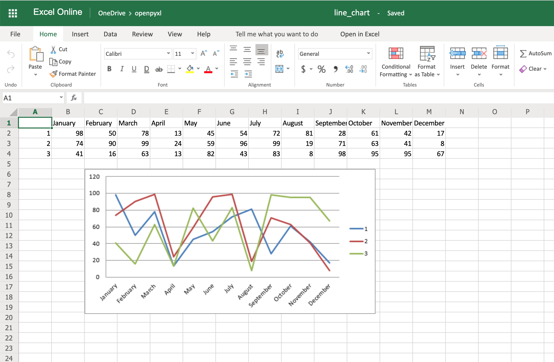
There are a couple of other things you can also change regarding the style of the chart. For example, you can add specific categories to the chart:

cats=Reference(worksheet=sheet,min_row=1,max_row=1,min_col=2,max_col=13)chart.set_categories(cats)

Add this piece of code before saving the workbook, and you should see the month names appearing instead of numbers:

Example Spreadsheet With Line Chart and Categories

Code-wise, this is a minimal change. But in terms of the readability of the spreadsheet, this makes it much easier for someone to open the spreadsheet and understand the chart straight away.

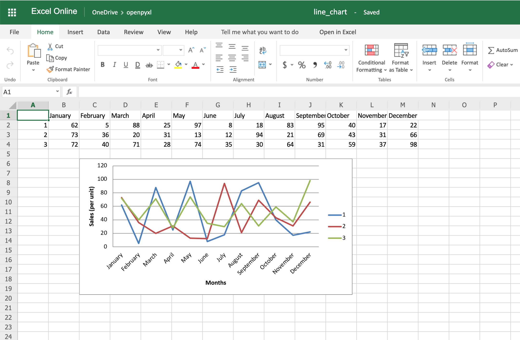
Another thing you can do to improve the chart readability is to add an axis. You can do it using the attributes x_axis and y_axis:

chart.x_axis.title="Months"chart.y_axis.title="Sales (per unit)"

This will generate a spreadsheet like the below one:

Example Spreadsheet With Line Chart, Categories and Axis Titles

As you can see, small changes like the above make reading your chart a much easier and quicker task.

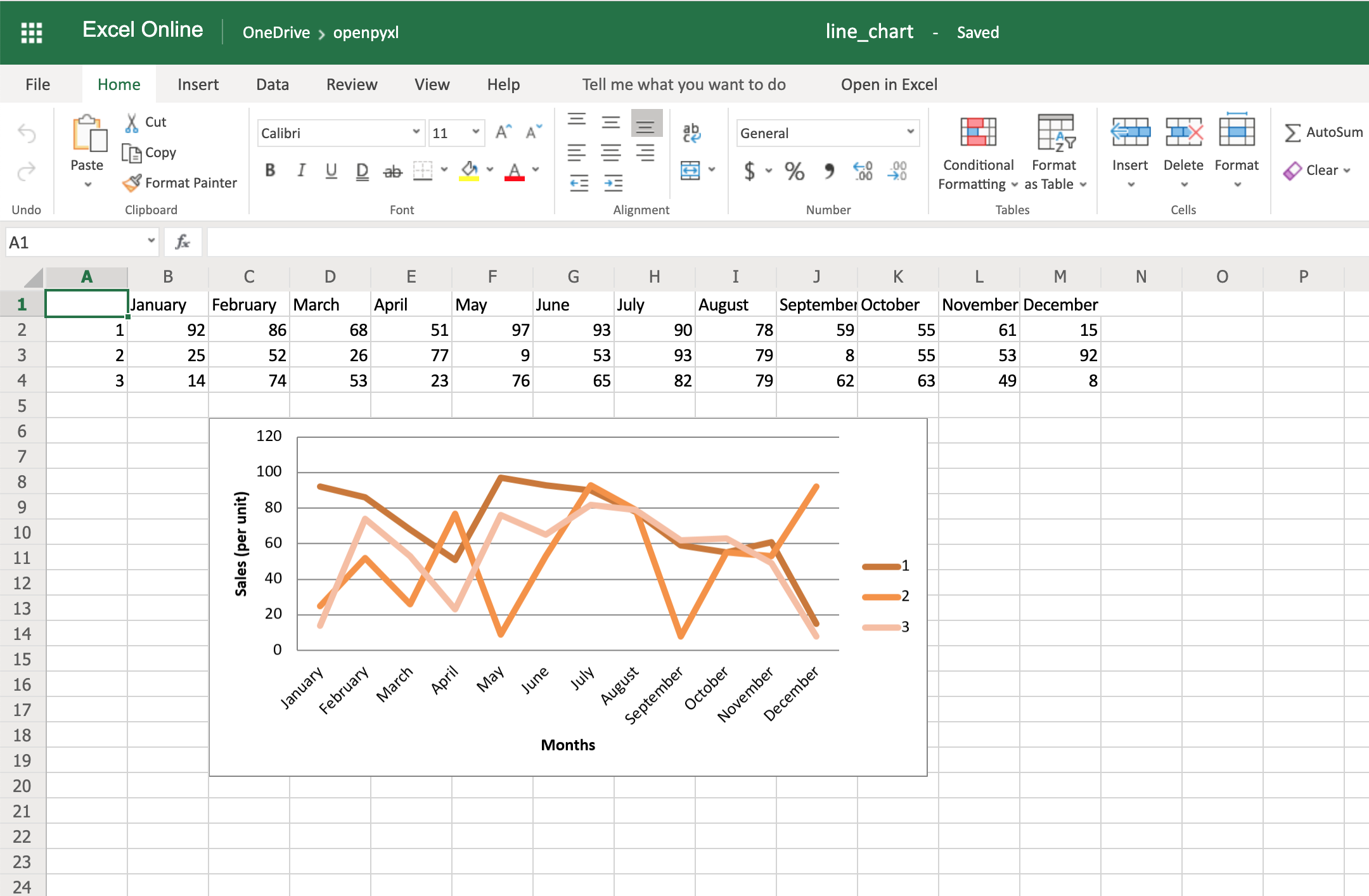
There is also a way to style your chart by using Excel’s default ChartStyle property. In this case, you have to choose a number between 1 and 48. Depending on your choice, the colors of your chart change as well:

# You can play with this by choosing any number between 1 and 48chart.style=24

With the style selected above, all lines have some shade of orange:

Example Spreadsheet With Line Chart, Categories, Axis Titles and Style

There is no clear documentation on what each style number looks like, but this spreadsheet has a few examples of the styles available.

Here’s the full code used to generate the line chart with categories, axis titles, and style:

importrandomfromopenpyxlimportWorkbookfromopenpyxl.chartimportLineChart,Referenceworkbook=Workbook()sheet=workbook.active# Let's create some sample sales datarows=[["","January","February","March","April","May","June","July","August","September","October","November","December"],[1,],[2,],[3,],]forrowinrows:sheet.append(row)forrowinsheet.iter_rows(min_row=2,max_row=4,min_col=2,max_col=13):forcellinrow:cell.value=random.randrange(5,100)# Create a LineChart and add the main datachart=LineChart()data=Reference(worksheet=sheet,min_row=2,max_row=4,min_col=1,max_col=13)chart.add_data(data,titles_from_data=True,from_rows=True)# Add categories to the chartcats=Reference(worksheet=sheet,min_row=1,max_row=1,min_col=2,max_col=13)chart.set_categories(cats)# Rename the X and Y Axischart.x_axis.title="Months"chart.y_axis.title="Sales (per unit)"# Apply a specific Stylechart.style=24# Save!sheet.add_chart(chart,"C6")workbook.save("line_chart.xlsx")

There are a lot more chart types and customization you can apply, so be sure to check out the package documentation on this if you need some specific formatting.

Convert Python Classes to Excel Spreadsheet

You already saw how to convert an Excel spreadsheet’s data into Python classes, but now let’s do the opposite.

Let’s imagine you have a database and are using some Object-Relational Mapping (ORM) to map DB objects into Python classes. Now, you want to export those same objects into a spreadsheet.

Let’s assume the following data classes to represent the data coming from your database regarding product sales:

fromdataclassesimportdataclassfromtypingimportList@dataclassclassSale:id:strquantity:int@dataclassclassProduct:id:strname:strsales:List[Sale]

Now, let’s generate some random data, assuming the above classes are stored in a db_classes.py file:

 1 importrandom 2  3 # Ignore these for now. You'll use them in a sec ;) 4 fromopenpyxlimportWorkbook 5 fromopenpyxl.chartimportLineChart,Reference 6  7 fromdb_classesimportProduct,Sale 8  9 products=[]10 11 # Let's create 5 products12 foridxinrange(1,6):13 sales=[]14 15 # Create 5 months of sales16 for_inrange(5):17 sale=Sale(quantity=random.randrange(5,100))18 sales.append(sale)19 20 product=Product(id=str(idx),21 name="Product %s"%idx,22 sales=sales)23 products.append(product)

By running this piece of code, you should get 5 products with 5 months of sales with a random quantity of sales for each month.

Now, to convert this into a spreadsheet, you need to iterate over the data and append it to the spreadsheet:

25 workbook=Workbook()26 sheet=workbook.active27 28 # Append column names first29 sheet.append(["Product ID","Product Name","Month 1",30 "Month 2","Month 3","Month 4","Month 5"])31 32 # Append the data33 forproductinproducts:34 data=[product.id,product.name]35 forsaleinproduct.sales:36 data.append(sale.quantity)37 sheet.append(data)

That’s it. That should allow you to create a spreadsheet with some data coming from your database.

However, why not use some of that cool knowledge you gained recently to add a chart as well to display that data more visually?

All right, then you could probably do something like this:

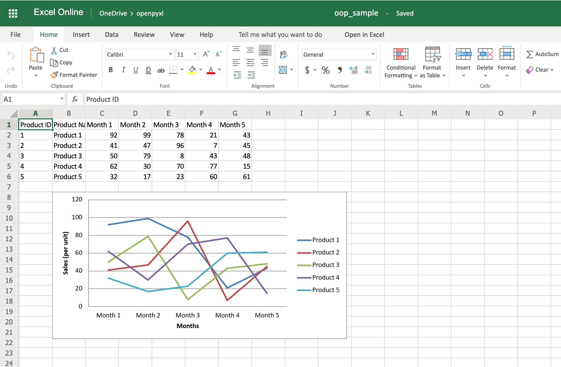
38 chart=LineChart()39 data=Reference(worksheet=sheet,40 min_row=2,41 max_row=6,42 min_col=2,43 max_col=7)44 45 chart.add_data(data,titles_from_data=True,from_rows=True)46 sheet.add_chart(chart,"B8")47 48 cats=Reference(worksheet=sheet,49 min_row=1,50 max_row=1,51 min_col=3,52 max_col=7)53 chart.set_categories(cats)54 55 chart.x_axis.title="Months"56 chart.y_axis.title="Sales (per unit)"57 58 workbook.save(filename="oop_sample.xlsx")

Now we’re talking! Here’s a spreadsheet generated from database objects and with a chart and everything:

Example Spreadsheet With Conversion from Python Data Classes

That’s a great way for you to wrap up your new knowledge of charts!

Bonus: Working With Pandas

Even though you can use Pandas to handle Excel files, there are few things that you either can’t accomplish with Pandas or that you’d be better off just using openpyxl directly.

For example, some of the advantages of using openpyxl are the ability to easily customize your spreadsheet with styles, conditional formatting, and such.

But guess what, you don’t have to worry about picking. In fact, openpyxl has support for both converting data from a Pandas DataFrame into a workbook or the opposite, converting an openpyxl workbook into a Pandas DataFrame.

Note: If you’re new to Pandas, check our course on Pandas DataFrames beforehand.

First things first, remember to install the pandas package:

$ pip install pandas

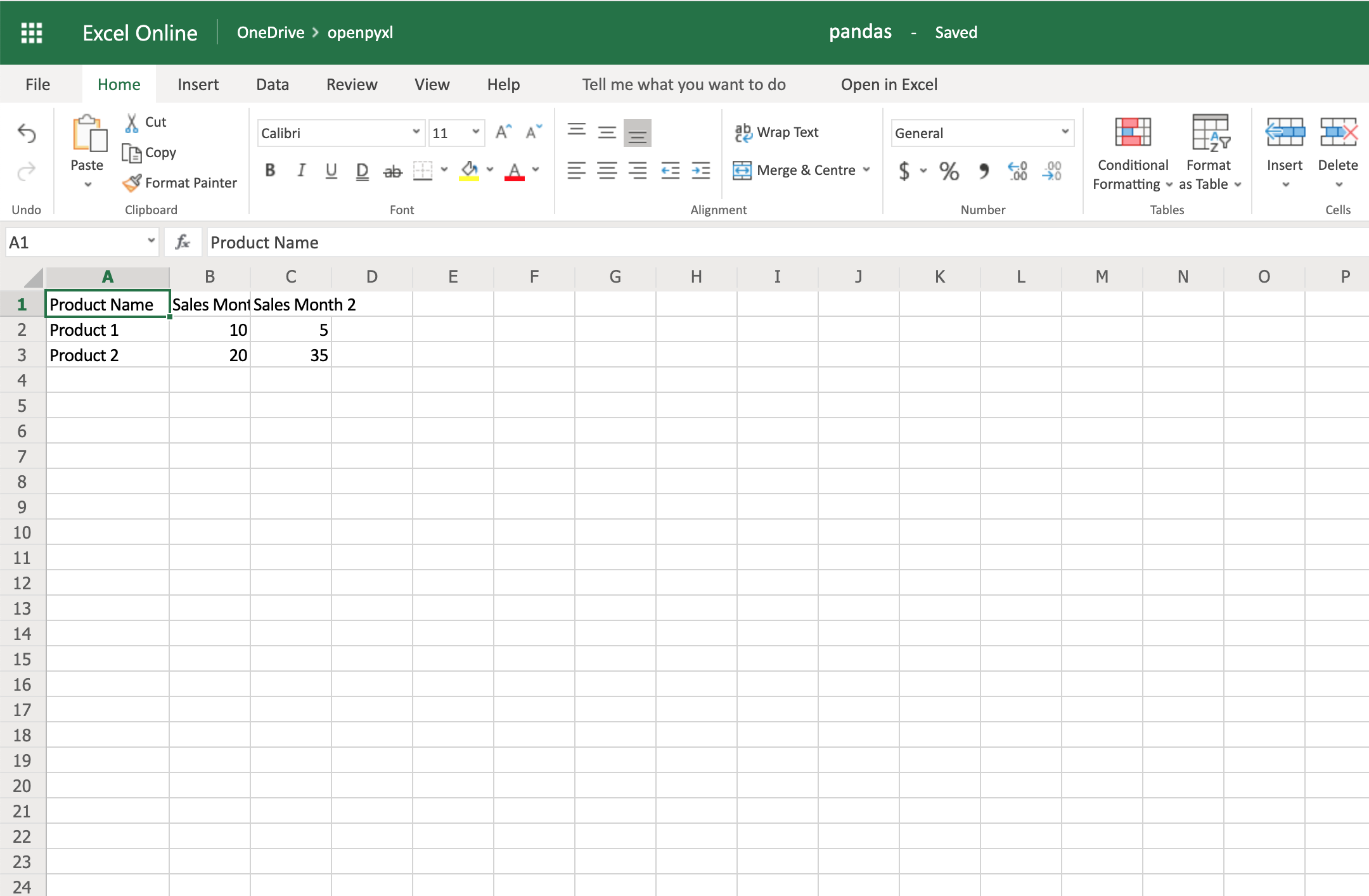
Then, let’s create a sample DataFrame:

 1 importpandasaspd 2  3 data={ 4 "Product Name":["Product 1","Product 2"], 5 "Sales Month 1":[10,20], 6 "Sales Month 2":[5,35], 7 } 8 df=pd.DataFrame(data)

Now that you have some data, you can use .dataframe_to_rows() to convert it from a DataFrame into a worksheet:

10 fromopenpyxlimportWorkbook11 fromopenpyxl.utils.dataframeimportdataframe_to_rows12 13 workbook=Workbook()14 sheet=workbook.active15 16 forrowindataframe_to_rows(df,index=False,header=True):17 sheet.append(row)18 19 workbook.save("pandas.xlsx")

You should see a spreadsheet that looks like this:

Example Spreadsheet With Data from Pandas Data Frame

If you want to add the DataFrame’s index, you can change index=True, and it adds each row’s index into your spreadsheet.

On the other hand, if you want to convert a spreadsheet into a DataFrame, you can also do it in a very straightforward way like so:

importpandasaspdfromopenpyxlimportload_workbookworkbook=load_workbook(filename="sample.xlsx")sheet=workbook.activevalues=sheet.valuesdf=pd.DataFrame(values)

Alternatively, if you want to add the correct headers and use the review ID as the index, for example, then you can also do it like this instead:

importpandasaspdfromopenpyxlimportload_workbookfrommappingimportREVIEW_IDworkbook=load_workbook(filename="sample.xlsx")sheet=workbook.activedata=sheet.values# Set the first row as the columns for the DataFramecols=next(data)data=list(data)# Set the field "review_id" as the indexes for each rowidx=[row[REVIEW_ID]forrowindata]df=pd.DataFrame(data,index=idx,columns=cols)

Using indexes and columns allows you to access data from your DataFrame easily:

>>>
>>> df.columnsIndex(['marketplace', 'customer_id', 'review_id', 'product_id',       'product_parent', 'product_title', 'product_category', 'star_rating',       'helpful_votes', 'total_votes', 'vine', 'verified_purchase',       'review_headline', 'review_body', 'review_date'],      dtype='object')>>> # Get first 10 reviews' star rating>>> df["star_rating"][:10]R3O9SGZBVQBV76    5RKH8BNC3L5DLF     5R2HLE8WKZSU3NL    2R31U3UH5AZ42LL    5R2SV659OUJ945Y    4RA51CP8TR5A2L     5RB2Q7DLDN6TH6     5R2RHFJV0UYBK3Y    1R2Z6JOQ94LFHEP    5RX27XIIWY5JPB     4Name: star_rating, dtype: int64>>> # Grab review with id "R2EQL1V1L6E0C9", using the index>>> df.loc["R2EQL1V1L6E0C9"]marketplace               UScustomer_id         15305006review_id     R2EQL1V1L6E0C9product_id        B004LURNO6product_parent     892860326review_headline   Five Starsreview_body          Love itreview_date       2015-08-31Name: R2EQL1V1L6E0C9, dtype: object

There you go, whether you want to use openpyxl to prettify your Pandas dataset or use Pandas to do some hardcore algebra, you now know how to switch between both packages.

Conclusion

Phew, after that long read, you now know how to work with spreadsheets in Python! You can rely on openpyxl, your trustworthy companion, to:

  • Extract valuable information from spreadsheets in a Pythonic manner
  • Create your own spreadsheets, no matter the complexity level
  • Add cool features such as conditional formatting or charts to your spreadsheets

There are a few other things you can do with openpyxl that might not have been covered in this tutorial, but you can always check the package’s official documentation website to learn more about it. You can even venture into checking its source code and improving the package further.

Feel free to leave any comments below if you have any questions, or if there’s any section you’d love to hear more about.


[ Improve Your Python With 🐍 Python Tricks 💌 – Get a short & sweet Python Trick delivered to your inbox every couple of days. >> Click here to learn more and see examples ]

PSF GSoC students blogs: Check-in: 13th and final week of GSoC (Aug 19 - Aug 25)

$
0
0

1. What did you do this week?

  • As this was the final week of GSoC, I have written and posted a final report of the project here.
  • In addition, I made a major overhaul of the project's website. Wich now contains a "gallery of examples" for some of major advancements and tools developed during the GSoC period.
  • See this PR for a more detailed list of contributions made this week.

2. What is coming up next?

  • There are a couple of open questions that concern the integration of these tools and analysis techniques to MNE's API.
  • For instance, we've been using scikit-learn's linear regression module to fit the models. One of the main advantages of this approach consists in having a linear regression "object" as output, increasing the flexibility for manipulation of the linear model results, while leaving MNE's linear regression function untouched (for now). However, we believe that using a machine learning package for linear regression might lead to confusion among users on the long run.
  • Thus, the next step is to discuss possible ways of integration to MNE-Python. Do we want to modify, simplify, or completely replace MNE's linear regression function to obtain similar output..

I really enjoyed working on this project during the summer and would be glad to continue working on extending the linear regression functionality of MNE-Python after GSoC.

3. Did you get stuck anywhere?

  • Not really. Although the final week included a lot of thinking about what the most practical API might be for the tools developed during the GSoC period. We want to continue this discussion online (see here) and hopefully be able to fully integrate this advancements in the released version of MNE-Python soon.

Thanks for reading and please feel free to contribute, comment or post further ideas!

PSF GSoC students blogs: Final Weekly Check-in

$
0
0

In the final week of coding, I was refining the hadoop source PR.

What did I do this week?

The dockerfile is finally working now. We are able to set up hadoop using dockerfile. Also the connection set up is well established in the application.

What is coming up next?

There are few bug fixes to be done. Also Hadoop feature and MySQL feature are going to be packaged and uploaded in PyPi similar to the models. I will be working on that as well.

Did you get stuck anywhere?

Fixing the hadoop source connection and writing a data into HDFS stream was an issue. My mentor and I had another meeting this week and we fixed it.

Podcast.__init__: AI Driven Automated Code Review With DeepCode

$
0
0
Software engineers are frequently faced with problems that have been fixed by other developers in different projects. The challenge is how and when to surface that information in a way that increases their efficiency and avoids wasted effort. DeepCode is an automated code review platform that was built to solve this problem by training a model on a massive array of open sourced code and the history of their bug and security fixes. In this episode their CEO Boris Paskalev explains how the company got started, how they build and maintain the models that provide suggestions for improving your code changes, and how it integrates into your workflow.

Summary

Software engineers are frequently faced with problems that have been fixed by other developers in different projects. The challenge is how and when to surface that information in a way that increases their efficiency and avoids wasted effort. DeepCode is an automated code review platform that was built to solve this problem by training a model on a massive array of open sourced code and the history of their bug and security fixes. In this episode their CEO Boris Paskalev explains how the company got started, how they build and maintain the models that provide suggestions for improving your code changes, and how it integrates into your workflow.

Announcements

  • Hello and welcome to Podcast.__init__, the podcast about Python and the people who make it great.
  • When you’re ready to launch your next app or want to try a project you hear about on the show, you’ll need somewhere to deploy it, so take a look at our friends over at Linode. With 200 Gbit/s private networking, scalable shared block storage, node balancers, and a 40 Gbit/s public network, all controlled by a brand new API you’ve got everything you need to scale up. And for your tasks that need fast computation, such as training machine learning models, they just launched dedicated CPU instances. Go to pythonpodcast.com/linode to get a $20 credit and launch a new server in under a minute. And don’t forget to thank them for their continued support of this show!
  • You listen to this show to learn and stay up to date with the ways that Python is being used, including the latest in machine learning and data analysis. For even more opportunities to meet, listen, and learn from your peers you don’t want to miss out on this year’s conference season. We have partnered with organizations such as O’Reilly Media, Dataversity, Corinium Global Intelligence, and Data Council. Upcoming events include the O’Reilly AI conference, the Strata Data conference, the combined events of the Data Architecture Summit and Graphorum, and Data Council in Barcelona. Go to pythonpodcast.com/conferences to learn more about these and other events, and take advantage of our partner discounts to save money when you register today.
  • Your host as usual is Tobias Macey and today I’m interviewing Boris Paskalev about DeepCode, an automated code review platform for detecting security vulnerabilities in your projects

Interview

  • Introductions
  • Can you start by explaining what DeepCode is and the story of how it got started?
  • How is the DeepCode platform implemented?
  • What are the current languages that you support and what was your guiding principle in selecting them?
    • What languages are you targeting next?
    • What is involved in maintaining support for languages as they release new versions with new features?
      • How do you ensure that the recommendations that you are making are not using languages features that are not available in the runtimes that a given project is using?
  • For someone who is using DeepCode, how does it fit into their workflow?
  • Can you explain the process that you use for training your models?
    • How do you curate and prepare the project sources that you use to power your models?
      • How much domain expertise is necessary to identify the faults that you are trying to detect?
      • What types of labelling do you perform to ensure that the resulting models are focusing on the proper aspects of the source repositories?
  • How do you guard against false positives and false negatives in your analysis and recommendations?
  • Does the code that you are analyzing and the resulting fixes act as a feedback mechanism for a reinforcement learning system to update your models?
    • How do you guard against leaking intellectual property of your scanned code when surfacing recommendations?
  • What have been some of the most interesting/unexpected/challenging aspects of building the DeepCode product?
  • What do you have planned for the future of the platform and business?

Keep In Touch

Picks

Closing Announcements

  • Thank you for listening! Don’t forget to check out our other show, the Data Engineering Podcast for the latest on modern data management.
  • Visit the site to subscribe to the show, sign up for the mailing list, and read the show notes.
  • If you’ve learned something or tried out a project from the show then tell us about it! Email hosts@podcastinit.com) with your story.
  • To help other people find the show please leave a review on iTunes and tell your friends and co-workers
  • Join the community in the new Zulip chat workspace at pythonpodcast.com/chat

Links

The intro and outro music is from Requiem for a Fish The Freak Fandango Orchestra / CC BY-SA

PSF GSoC students blogs: Final work submission and future work

$
0
0

As the final week ended, we had to submit a compilation of our work during GSoC. Below are some insights:

What was the original aim?

Adding new machine learning models to DFFML, the proposed models are given below:

  1. Model 1: Ordinary Least Square Regression (OLSR)
  2. Model 2: Logistic Regression
  3. Model 3: k-Nearest Neighbour (kNN)
  4. Model 4: Naive Bayes

Decided modifications during community bonding:

During the community bonding period, the proposed work was modified to achieve optimized result from the summer. The finalized work was:

  1. Adding Linear Regression Model from scratch
  2. Adding Linear Regression and other proposed models using scikit-learn
  3. Adding tests for the added models
  4. Documenting the models

Tasks Completed:

  • Added Linear Regression model from scratch with tests

    Simple Linear Regression model implemented from scratch. This was successfully completed with tests and documentation, and was also releasd on PyPI.

  • Added scikit models with dynamic support Initially, it was planned to add certain number of models from scikit but as I did it with one model (Multiple Linear Regression with scikit), we decided to extend this and make a base for all scikit models and make other model classes dynamic. This was successful and now adding scikit models to DFFML is as easy as appending the model name to a python dictionary. The tests are complete and the documentation material is ready but we are still figuring out a more understandable way of documenting this before release.

Future Work:

The project was started just before GSoC'19 and it has come a long way since. I plan on contributing significantly to the project after GSoC'19. Few of the planned stuff:

  1. Adding more scikit models
  2. Working on more machine learning libraries and add models
  3. Contruct DFFML Web UI from scratch which was conceptualized during summer and much more.


More detailed report: https://gist.github.com/yashlamba/5e0845a6cd5a1198f166ddedfba78802


Viewing all 22871 articles
Browse latest View live


<script src="https://jsc.adskeeper.com/r/s/rssing.com.1596347.js" async> </script>