Quantcast
Channel: Planet Python
Viewing all 22646 articles
Browse latest View live

Continuum Analytics Blog: Who You Gonna Call? Halloween Tips & Treats to Protect You from Ghosts, Gremlins…and Software Vulnerabilities

$
0
0

By Michael Sarahan Happy Halloween, readers. At Anaconda, we’re not too scared about things that go bump in the night. We’ve examined the data and concluded that it’s just the cleaning staff upstairs. We are, however, kept awake by the ever-present concern of the security and experience of our users! We’d like to take this …
Read more →

The post Who You Gonna Call? Halloween Tips & Treats to Protect You from Ghosts, Gremlins…and Software Vulnerabilities appeared first on Anaconda.


Erik Marsja: Repeated Measures ANOVA in Python using Statsmodels

$
0
0

In this brief Python data analysis tutorial we will learn how to carry out a repeated measures ANOVA using Statsmodels. More specifically, we will learn how to use the AnovaRM class from statsmodels anova module.

To follow this guide you will need to have Python, Statsmodels, Pandas, and their dependencies installed. One easy way to get these Python packages installed is to install a Python distribituion such as Anaconda (see this YouTube Video on how to install Anaconda). However, if you already have Python installed you can of course use Pip.

How to carry out repeated measures ANOVA using other Python packages:

This short tutorial are devided so that we will learn how to install Statsmodels and Pandas, carrying out one-way and two-way ANOVA using statsmodels. Finally, there is a YouTube video showing how to carry out repeated measures ANOVA using Statsmodels and R. This Youtube video will also show some of the differences between Statsmodel and the r-package afex and the function aov_ez.

How to Install Statsmodels & Pandas

Statsmodels and Panda can easily be installed using pip:

pip install pandas statsmodels

How to Use AnovaRM to Carry Out a Repeated Measures ANOVA

In this section we are going to learn how to do a repeated measures ANOVA using Statsmodels. More specifically, we are going to learn how carry out a one-way ANOVA and two-way ANOVA in Python. The AnovaRM clas takes five arguments:

  • data: the first argument should be a dataframe object.
  • depvar: second should variable should be your dependent variable. Should be a string (e.g., ‘responsetime’)
  • subject: here you put in your subject identifier. Should also be a string (e.g., ‘subject’)
  • within:  the within-subject factors in a lit of strings.
  • aggregate_func: this is optional and should be use if the data contains more than a single observation per participant. Can be “mean” or a function. For instance, you can use Numpy mean (i.e., np.mean).

One-way ANOVA for Repeated Measures Using Statsmodels

First we start with the one-way ANOVA. In the examples below we are going to use Pandas and the AnovaRM class from statsmodels. In the first example, we are using Pandas to use read_csv to load this data into a dataframe. See my Python Pandas Dataframe tutorial if you need to learn more about Pandas dataframes.

import pandas as pd
from statsmodels.stats.anova import AnovaRM

df = pd.read_csv('rmAOV1way.csv')

We can use Pandas head() to have a look at the first five row (i.e., df.head()):

First 5 rows of the Pandas dataframe.

As can be seen above we have the columns Sub_id, rt, and cond. These columns represent the subject identifier, the dependent variable, and the independent variable, respectively. Note, there are two levels of cond (using df.cond.unique() will show us noise and quiet).

Python One-way Repeated Measures ANOVA Example:

In the Statsmodels ANOVA example below we use our dataframe object, df, as the first argument, followed by our independent variable (‘rt’), subject identifier (‘Sub_id’), and the list of the dependend variable, ‘cond’. In the second row we are getting the fit so that we can print the ANOVA table.

aovrm = AnovaRM(df, 'rt', 'Sub_id', within=['cond'])
res = aovrm.fit()

print(res)

Output: ANOVA table

In the second example we will also use the parameter aggregate_func. Click here to download the dataset.

flanks = pd.read_csv('flanks.csv')
res = AnovaRM(flanks, 'RT', 'SubID', within=['TrialType'], aggregate_func='mean')

print(res.fit())

Two-way ANOVA for Repeated Measures Using Statsmodels

Finally, we continue with the two-way ANOVA. In the example below we are also using Pandas and the AnovaRM class from statsmodels. The example data can be downloaded here.

Two-Way ANOVA Using Statsmodels Example:

Notice the difference between the one-way ANOVA and the two-way ANOVA; the list now contains 2 variables.

df2way = pd.read_csv('rmAOV2way.csv')
aovrm2way = AnovaRM(df2way, 'rt', 'Sub_id', within=['iv1', 'iv2'])
res2way = aovrm2way.fit()

print(res2way)

The ANOVA table when carrying out a two-way ANOVA using Statsmodels look like this:

ANOVA Table Statmodels

Repeated Measures ANOVA: R vs. Python

Finally, here’s the YouTube video covering how to carry out repeated measures ANOVA using Python and R. It will further show some of the differences between the function aov_ez and AnovaRM. Hint, there are more arguments available in aov_ez and it will calculate effect sizes, among other things.

That was it, now you know how to carry out one-way and two-way ANOVA for repeated measures using Python Statsmodels.

The post Repeated Measures ANOVA in Python using Statsmodels appeared first on Erik Marsja.

Python Bytes: #102 Structure of a Flask Project

Karim Elghamrawy: Python: Let’s Create a Simple HTTP Server (Tutorial)

$
0
0

Web severs are everywhere. Heck you are interacting with one right now! No matter what type of software engineer you are, at some point in your career you will have to interact with web servers. May be you are building an API server for a backend service. Or may be you are just configuring a [...]

The post Python: Let’s Create a Simple HTTP Server (Tutorial) appeared first on Afternerd.

Techiediaries - Django: React 16.7 Hooks — with Axios and Django API [PART 1]

$
0
0

React Hooks are a new feature recently released by the React team. It's included in React 16.7 which is in its Alpha version as of this writing.

React Hooks Tutorial

In this tutorial, we'll learn to migrate our previous project created with React and Django to use function components and React Hooks instead of class components, life-cycle methods and the state object.

Prerequisites

You need to have:

  • Python 3, Pip and venv installed for running the back-end API,
  • Node.js 6+, npm 5.2+ and create-react-app for running the React app,
  • Git for cloning our project from GitHub.

Cloning and Setting Up our React/Django Project

First let's start by cloning our full-stack React/Django project.

Navigate to your home directory and create a virtual environment using the venv module:

$ cd ~
$ python3 -m venv ./env

Activate the created virtual environment using:

$ source env/bin/activate

Using Git run the following command from your terminal:

$ git clone https://github.com/techiediaries/django-react.git django-react-hooks

Next, navigate to your cloned project using:

$ cd django-react-hooks

Next install the dependencies using pip:

$ pip install django djangorestframework django-cors-headers

Now, navigate to the frontend folder and install the dependencies using npm:

$ cd frontend
$ npm install

This will install React and Axios.

Since, we need to use React Hooks; we have to install the latest version of React which is react@16.7.0-alpha.0.

You simply need to run the following commands:

$ npm install react@16.7.0-alpha.0 --save
$ npm install react-dom@16.7.0-alpha.0 --save

This will install the latest react and react-dom alpha versions which support React Hooks.

Introduction to React Hooks

Before migrating our demo project to functional components and React Hooks let's first understand what hooks are and why we need to use them.

So why all that buzz about React hooks? And what can they do for you?

Simply, if you need to use React features like state and life-cycle events/methods (which is often most of the times) you would need to use/switch to classes by extending React.Component. But, that's not the case any more; with hooks you can now use those commonly needed features in your functional components.

What is A React Hook?

React is nowadays the most popular and used UI library in the world. The team is constantly trying to improve both the performance of the library and the developer experience by adding new features that makes developer's lives more easy.

As of this writing, most React developers are very existed about a new React feature -- Hooks, they are now on alpha version and they will be included in React 16.7.

A React Hook is a new feature (that's only available in alpha as of this writing) to use the React.Component features in a functional component.

The most used features are:

  • The state object,
  • Life-cycle events like componentWillMount, componentDidMount, componentWillUpdate and componentDidUpdate etc.
  • context,
  • refs etc.

Saying that, class-based components are still useful. It's just that you have now more options to do the same thing and It's up to your preferences to use either classes or functions to build your React apps without being limited by the lack of features with any option.

Just like with the other React concepts; they have fancy names but they are actually simple concepts to understand. Hooks are also simple functions that allow developers to “hook into” React state and life-cycle methods from functional components. Hooks are not available in class-based components — bu instead they allow you to use React without JavaScript classes. If you prefer to use functions instead of classes (which is recommended in JavaScript) you can simply start using Hooks without worrying about migrating your whole apps to classes.

Hooks enables you to use “class-features” In React by providing a set of built-in functions such as:

  • The useState() hook for using states from function components,
  • The useEffect() hook for performing side effects from function components (it's equivalent to life-cycle methods like componentDidMount, componentDidUpdate, and componentWillUnmount in React classes),

  • The useContext() hook for subscribing to React Context from a function component,

  • The useReducer() hook for managing the state of components with a reducer

  • useRef for React Refs,

  • The useCallback hook for callbacks,

  • The useMemo hook for memoized values,

  • The useImperativeMethods hook for imperative methods,

  • The useMutationEffect hook for mutation effects,

  • The useLayoutEffect hook for layout effects.

You can also create your custom Hooks to re-use any stateful behavior between different components.

In other words Hooks lets you have stateful functional components.

React Hooks are typical JavaScript functions, with the exception that they need to obey to two rules:

  • Hooks need to be used at the top level i.e not inside nested functions or other JS constructs like loops or if conditions etc.
  • Hooks need to be used in functional components not in regular JavaScript functions. You can also call built-in Hooks from your custom Hooks

The React team provides a linter plugin that can be used by developers to make sure these rules are respected so Hooks can work as expected in your app.

Example Accessing State in Functions with useState()

Now that we have seen some theory about React Hooks. Let’s see a simple example of a stateful function component with the useState() hook. Let’s start with a simple stateless function component that we are familiar with.

This a simple React app with one ContactPage function component:

importReactfrom'react';import{render}from'react-dom';functionContactPage(props){return(<div><h1>ContactPage</h1>
</div>);
}render(<ContactPage/>,document.querySelector('#root'));

In the old React, If we want to keep or work with any state in this component we'll need to convert it into a class component. For example, let's say we need to use an email variable in our component. This is what we'll have to do:

classContactPageextendsReact.Component{state={email:'a@email.com'}render(){return(<div><h1>ContactPage</h1>
<p>Myemailis{this.state.email}</p>
</div>
);}}

We rewrite our component to use a class instead of a function so we can be able to use the state object.

Now, thanks to React Hooks we can simply use this alternative code without re-writing you component:

importReact,{useState}from'react';import{render}from'react-dom';functionContactPage(props){const[email,setEmail]=useState('a@email.com');return(<div><h1>ContactPage</h1>
<p>Myemailis{this.state.email}</p>    </div>);
}

This is our regular function but it's now equipped with a state using the useState() hook function.

Note that hook functions start with the use word which is another rule of Hooks.

The useState() hook takes an initial state and returns an array with two elements: the current state, and a function to set the state. In our example, we pass in the a@email.com string as initial state
and we use array destructing assignment to grab variables and rename them properly. We can access the current piece of state using email and the function to set the state using setEmail.

The useState() hook provides us with two variables that we need to rename with proper names. To be able to rename these variables properly, you need to know these two things:

  • The first element of the returned array presents the value which equivalent to this.state in class components.
  • The second element is a function to set that value which is equivalent to this.setState() in classes.

The state can be any valid JavaScript object.

React functional components have no state, but thanks to the useState() hook we can have little pieces of state when we need them.

Example using The Effect Hook in React

Now that we have seen the State Hook with example and understand why we need to use it - which is to lets us use state in React functional components. Let's see an example using the Effect Hook to be able to perform side effects in our functional components without resorting to use life-cycle methods which are only available in class components.

Effect Hooks are equivalent to componentDidMount, componentDidUpdate and componentWillUnmount life-cycle methods.

Side effects are common operations that most web applications need to perform, such as:

  • Fetching and consuming data from a server API,
  • Updating the DOM,
  • Subscribing to Observables etc.

Effect Hooks will run after every render, including the first render.

importReact,{useState}from'react';functionCustomers(){const[customers,setCustomers]=useState([]);useEffect(()=>{fetch('127.0.0.1:8000/customers').then(response=>response.json()).then(data=>{setCustomers(data);// set customers in state});},[]);}

We first use the useState() with an empty array for the initial state to create a customers state.

Next, we'll use the useFetch() hook to run a side effect which is sending a request, using the Fetch API, to an API endpoint that returns a list of customers.

We finally use the setCustomers() method to assign the returned data to the customers state variable.

Conclusion

You can combine many types of hooks or use the same hook multiple times in your application without any problem. In fact, in most apps, you'll have to use them both in order to be able to fully use functional components without resorting to any feature in class components.

In the next part, we'll see a real-world example of using React Hooks with Axios and a Django API.

Tryton News: Newsletter November 2018

$
0
0

@ced wrote:

We have a fresh new website to better show the features of Tryton and be more speaking to the visitor. This has been possible thanks to the investment of the Foundation (meaning the donors). So do not forget to check our new donation page. :wink:

Contents:

Changes for the user

The stock_consignment module now supports internal shipment between supplier and customer. In this case the stock move creates two invoices. And it uses the origin of the invoice lines to manage them from the move workflow.

The notification_email module now allows employees as recipients, as it is quite common to have employees linked to documents (e.g. shipments).

Now it is possible to refund an invoice which already include partial payments. Refunding is possible, as long as there are no reconciled move lines. The state of a refunded invoice is now set to cancelled instead of paid.
This is an important change for a sale with shipment method set to on invoice paid. The resulted invoice is already posted, but should be refunded by a credit note. Now the state of the invoice is set to cancelled and the sale is set to invoice exception, instead of creating a most likely wrong shipment.

The drag & drop of file functionality on the web and desktop client is unified. On the web client, it is possible to drop file on the attachment button of the web client. And the desktop client supports dropping file on the binary widgets.

Entering time sheets from the project is simplified as the work is filled automatically.

New Module implementing user roles

The user_role module allows to assign roles to users. Roles are sets of access groups. When a role is added to a user, it overrides existing groups. A role can be added to a user for a period.
This module is useful for large companies with complex access rights which evolve over time.

Changes for the developer

Now creating and deleting a note or attachment is checked only for write access permissions. The implementation provides an easy way to modify one type of check into another, if needed.

Posts: 1

Participants: 1

Read full topic

Rene Dudfield: Josh Bartlett — pygame Artist in Residence

$
0
0
The pygame Artist in Residence grant celebrates the Python arts community and lends a tiny bit of support to someones art practice. Josh Bartlett was the first recipient.

An artist residency usually works something like; a person spends some time in either a gallery making something to present or in a music club doing a weekly spot. The pygame artist in residence will do it in their own space, but be present on the top of the pygame website in the form of a thumbnail and a link to their patreon/blog/artist statement/website/whatever.

Josh Bartlett was the first recipient, and has been featured on the pygame website in October.  Please see the pygame artist in residence profile page for more info.


What has he been up to?  Go to his blog to find out.

ps. Thank you to everyone who applied, and those who helped with selection. Hopefully the next one will go more smoothly as the process is improved.

Made With Mu: Mu and PyWeek: Traffic Flowmageddon

$
0
0

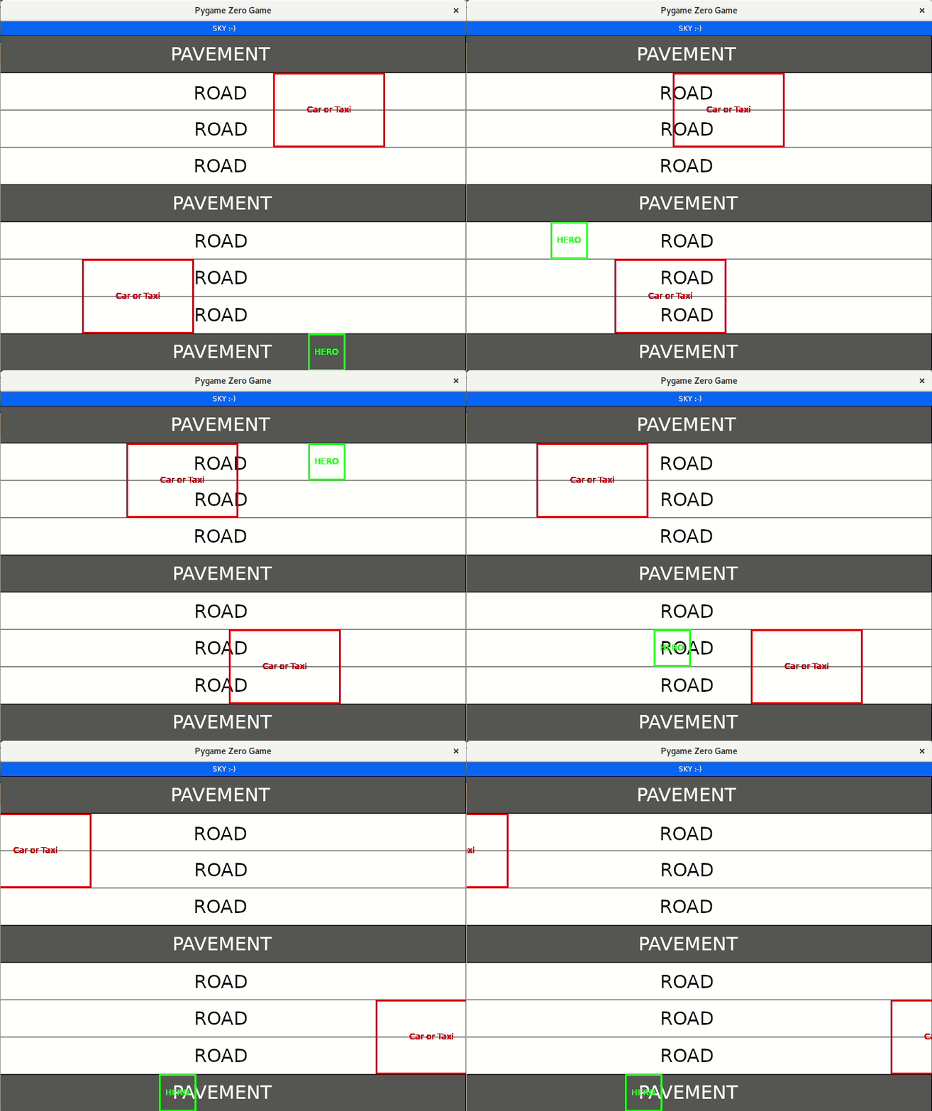
Last week was PyWeek, where entrants have a week to make a game on a given theme using Python. Myself and my buddy Andrew Smith decided to form a team called Code to Joy and write something using Mu and PyGameZero. At the start of the week the theme was revealed as “flow”. We ended up creating “Traffic Flowmageddon” with gameplay like 80’s classic Frogger, a look similar to the 90’s classic Grand Theft Auto and with a dash of Shaun of the Dead thrown in for some timely Halloween spice. The opening screen pretty much sums up the character of the game:

It was fun to work in a team. I mainly concentrated on the code and Andrew spent time on the sound effects and music. The graphical assets were either bodged together by us or were free-to-use downloads from the internet. What was particularly pleasing was how quickly we were able to put together the scaffolding of the game in a very short period of time and just under 100 lines of Python:

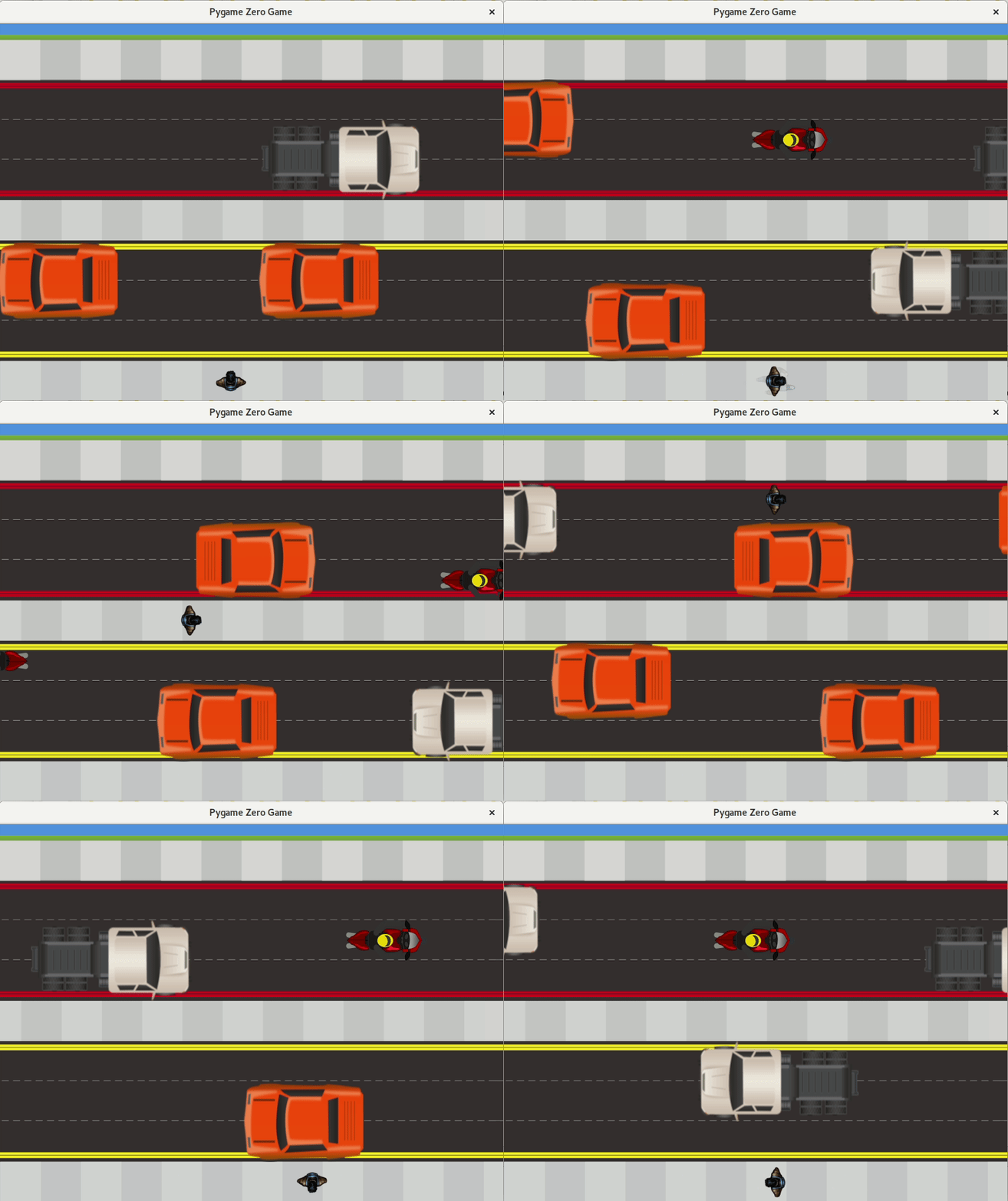
Yes, that’s quite an abstract looking game (none of the graphical assets had been created), but the labelled boxes and fact that stuff is moving around demonstrated the core of the game worked well. Having said that, simply adding some proper graphics and an animation on the hero sprite that the player controls makes a huge difference! It actually looks like a game:

At this point in the development of the game, one of us had the idea of adding zombies and, since I’d been tweeting about our progress, we were getting suggestions for other features from friends (such as potholes in the road which would slow you down, or drivers with no lane discipline).

The zombies make a big difference since they force you off the pavement and into the flow of traffic.

In the meantime, Andrew had been putting together music and sound effects as well as the code to load and play them at the appropriate moments in the game. This was especially rewarding to hear since sound and music add so much to the atmosphere. Andrew found some appropriately spooky sounding music, a “happy tune” to play when the game completed and a whole host of sounds for the zombies and traffic (for example, if you get too close to one of the London taxi cabs, the driver will shout at you).


As the video shows, the finished game works quite well for something cobbled together in just a week. Most importantly, it’s all done with Mu and PyGameZero in around 400 lines of Python.

I’d heartily recommend anyone participate in future PyWeeks. The organiser, Dan Pope (who also created PyGameZero) has done a fantastic job of creating such a fun competition with a community of coders creating such joyously goofy games.

Long may it last!


PyCharm: PyCharm 2018.3 EAP 9

$
0
0

We’ve entered the final phase of the Early Access Program (EAP) for PyCharm 2018.3, the ninth version is now available. Download this version from our website

New in This Version

Enhanced GitHub Integration

GitHub

We’ve included a couple of cool GitHub specific features in PyCharm. You can now update your fork of GitHub projects you contribute to right from PyCharm, then do some work, and create a pull request.

Do you maintain a project? You can now check out pull requests in PyCharm, and check out a branch to play with it right from the version control tools in your IDE.

Further Improvements

  • The Python 3.7 breakpoint() statement will now trigger the PyCharm debugger to break. Of course, you can still use regular breakpoints and prevent yourself from accidentally checking in a debugging statement.
  • A bug that caused Gtk to not have code completion has been resolved.
  • Sometimes when opening a task in PyCharm, the IDE would freeze for a long time, this has been resolved now. Did you know that PyCharm integrates with your issue tracker? Read more in our docs
  • And more, check out the release notes for more details

Interested?

Download this EAP from our website. Alternatively, you can use the JetBrains Toolbox App to stay up to date throughout the entire EAP.

If you’re on Ubuntu 16.04 or later, you can use snap to get PyCharm EAP, and stay up to date. You can find the installation instructions on our website.

PyCharm 2018.3 is in development during the EAP phase, therefore not all new features are already available. More features will be added in the coming weeks. As PyCharm 2018.3 is pre-release software, it is not as stable as the release versions. Furthermore, we may decide to change and/or drop certain features as the EAP progresses.

All EAP versions will ship with a built-in EAP license, which means that these versions are free to use for 30 days after the day that they are built. As EAPs are released weekly, you’ll be able to use PyCharm Professional Edition EAP for free for the duration of the EAP program, as long as you upgrade at least once every 30 days.

Dataquest: Python vs R: Head to Head Data Analysis

$
0
0

Which is better for data analysis?

There have been dozens of articles written comparing Python and R from a subjective standpoint. We'll add our own views at some point, but this article aims to look at the languages more objectively. We'll analyze a dataset side by side in Python and R, and show what code is needed in both languages to achieve the same result. This will let us understand the strengths and weaknesses of each language without the conjecture. At Dataquest, we teach both languages, and think both have a place in a data science toolkit.

We'll be analyzing a dataset of NBA players and their performance in the 2013-2014 season. You can download the file here. For each step in the analysis, we'll show the Python and R code, along with some explanation and discussion of the different approaches. Without further ado, let's get this head to head Python vs R matchup started!

Importing a CSV

R

library(readr)
nba <- read_csv("nba_2013.csv")

Python

import pandas
nba = pandas.read_csv("nba_2013.csv")

The above code will load the CSV file nba_2013.csv, which contains data on NBA players from the 2013-2014 season, into the variable nba in both languages. The only real difference is that in Python, we need to import the pandas library to get access to Dataframes. In R, while we can import the data using the base R function read.csv(), using the readr library function read_csv() has the advantage of greater speed and consistent interpretation of data types. Dataframes are available in both R and Python, and are two-dimensional arrays (matrices) where each column can be of a different datatype. At the end of this step, the CSV file has been loaded by both languages into a dataframe.

Finding the number of rows

R

dim(nba)
[1] 481  31

Python

nba.shape
(481, 31)

This prints out the number of players and the number of columns in each. We have 481 rows, or players, and 31 columns containing data on the players.

Looking at the first row of the data

R

head(nba, 1)
player pos age bref_team_id
1 Quincy Acy  SF  23          TOT
[output truncated]

Python

nba.head(1)
player pos  age bref_team_id
0  Quincy Acy  SF   23          TOT
[output truncated]

This is pretty much identical. Both print out the first row of the data, and the syntax is very similar. Python is more object-oriented here, and head is a method on the dataframe object, and R has a separate head function. This is a common theme you'll see as you start to do analysis with these languages, where Python is more object-oriented, and R is more functional.

Find the average of each statistic

Let's find the average value for each statistic. The columns, as you can see, have names like fg (field goals made), and ast (assists). These are the season statistics for the player. If you want a fuller explanation of all the stats, look here.

R

library(purrr)
library(dplyr)

nba %>%
  select_if(is.numeric) %>%
map_dbl(mean, na.rm = TRUE)
player NA
pos NA
age 26.5093555093555
bref_team_id NA
[output truncated]

Python

nba.mean()
age             26.509356
g               53.253638
gs              25.571726
[output truncated]

There are some major differences in approach here. In both, we're applying a function across the dataframe columns. In Python, the mean method on dataframes will find the mean of each column by default.

In R, we can use functions from two popular packages to select the columns we want to average and apply the mean function to them. The %>% operator, referred to as "the pipe", passes output of one function as input to the next. Taking the mean of string values will just result in NA -- not available. We can take the mean of only the numeric columns by using select_if. However, we do need to ignore NA values when we take the mean (requiring us to pass na.rm=TRUE into the mean function). If we don't, we end up with NA for the mean of columns like x3p.. This column is three point percentage. Some players didn't take three point shots, so their percentage is missing. If we try the mean function in R, we get NA as a response, unless we specify na.rm=TRUE, which ignores NA values when taking the mean. The .mean() method in Python already ignores these values by default.

Make pairwise scatterplots

One common way to explore a dataset is to see how different columns correlate to others. We'll compare the ast, fg, and trb columns.

R

library(GGally)

nba %>% 
  select(ast, fg, trb) %>%
  ggpairs()

r_pairs

Python

import seaborn as sns
import matplotlib.pyplot as plt
sns.pairplot(nba[["ast", "fg", "trb"]])
plt.show()

python_pairs

We get very similar plots in the end, but this shows how the R data science ecosystem has many smaller packages (GGally is a helper package for ggplot2, the most-used R plotting package), and many more visualization packages in general. In Python, matplotlib is the primary plotting package, and seaborn is a widely used layer over matplotlib. With visualization in Python, there is usually one main way to do something, whereas in R, there are many packages supporting different methods of doing things (there are at least a half dozen packages to make pair plots, for instance).

Make clusters of the players

One good way to explore this kind of data is to generate cluster plots. These will show which players are most similar.

R

library(cluster)
set.seed(1)
isGoodCol <- function(col){
   sum(is.na(col)) == 0 && is.numeric(col) 
}
goodCols <- sapply(nba, isGoodCol)
clusters <- kmeans(nba[,goodCols], centers=5)
labels <- clusters$cluster

Python

from sklearn.cluster import KMeans
kmeans_model = KMeans(n_clusters=5, random_state=1)
good_columns = nba._get_numeric_data().dropna(axis=1)
kmeans_model.fit(good_columns)
labels = kmeans_model.labels_

In order to cluster properly, we remove any non-numeric columns, or columns with missing values (NA, Nan, etc). In R, we do this by applying a function across each column, and removing it if it has any missing values or isn't numeric. We then use the cluster package to perform k-means and find 5 clusters in our data. We set a random seed using set.seed to be able to reproduce our results.

In Python, we use the main Python machine learning package, scikit-learn, to fit a k-means clustering model and get our cluster labels. We perform very similar methods to prepare the data that we used in R, except we use the get_numeric_data and dropna methods to remove non-numeric columns and columns with missing values.

Plot players by cluster

We can now plot out the players by cluster to discover patterns. One way to do this is to first use PCA to make our data 2-dimensional, then plot it, and shade each point according to cluster association.

R

nba2d <- prcomp(nba[,goodCols], center=TRUE)
twoColumns <- nba2d$x[,1:2]
clusplot(twoColumns, labels)

r_clus

Python

from sklearn.decomposition import PCA
pca_2 = PCA(2)
plot_columns = pca_2.fit_transform(good_columns)
plt.scatter(x=plot_columns[:,0], y=plot_columns[:,1], c=labels)
plt.show()

python_clus

Made a scatter plot of our data, and shaded or changed the icon of the data according to cluster. In R, the clusplot function was used, which is part of the cluster library. We performed PCA via the pccomp function that is built into R.

With Python, we used the PCA class in the scikit-learn library. We used matplotlib to create the plot.

Split into training and testing sets

If we want to do supervised machine learning, it's a good idea to split the data into training and testing sets so we don't overfit.

R

trainRowCount <- floor(0.8 * nrow(nba))
set.seed(1)
trainIndex <- sample(1:nrow(nba), trainRowCount)
train <- nba[trainIndex,]
test <- nba[-trainIndex,]

Python

train = nba.sample(frac=0.8, random_state=1)
test = nba.loc[~nba.index.isin(train.index)]

You'll notice that R has many more data-analysis focused builtins, like floor, sample, and set.seed, whereas these are called via packages in Python (math.floor, random.sample, random.seed). In Python, the recent version of pandas came with a sample method that returns a certain proportion of rows randomly sampled from a source dataframe -- this makes the code much more concise. In R, there are packages to make sampling simpler, but aren't much more concise than using the built-in sample function. In both cases, we set a random seed to make the results reproducible.

Univariate linear regression

Let's say we want to predict number of assists per player from field goals made per player.

R

fit <- lm(ast ~ fg, data=train)
predictions <- predict(fit, test)

Python

from sklearn.linear_model import LinearRegression
lr = LinearRegression()
lr.fit(train[["fg"]], train["ast"])
predictions = lr.predict(test[["fg"]])

Scikit-learn has a linear regression model that we can fit and generate predictions from. R relies on the built-in lm and predict functions. predict will behave differently depending on the kind of fitted model that is passed into it -- it can be used with a variety of fitted models.

Calculate summary statistics for the model

R

summary(fit)
Call:
lm(formula = ast ~ fg, data = train)

Residuals:
Min      1Q  Median      3Q     Max 
-228.26  -35.38  -11.45   11.99  559.61
[output truncated]

Python

import statsmodels.formula.api as sm
model = sm.ols(formula='ast ~ fga', data=train)
fitted = model.fit()
fitted.summary()


OLS Regression Results

Dep. Variable: ast
R-squared: 0.568
Model: OLS
Adj. R-squared: 0.567
[output truncated]

If we want to get summary statistics about the fit, like r-squared value, we'll need to do a bit more in Python than in R. With R, we can use the built-in summary function to get information on the model. With Python, we need to use the statsmodels package, which enables many statistical methods to be used in Python. We get similar results, although generally it's a bit harder to do statistical analysis in Python, and some statistical methods that exist in R don't exist in Python.

Fit a random forest model

Our linear regression worked well in the single variable case, but we suspect there may be nonlinearities in the data. Thus, we want to fit a random forest model.

R

library(randomForest)
predictorColumns <- c("age", "mp", "fg", "trb", "stl", "blk")
rf <- randomForest(train[predictorColumns], train$ast, ntree=100)
predictions <- predict(rf, test[predictorColumns])

Python

from sklearn.ensemble import RandomForestRegressor
predictor_columns = ["age", "mp", "fg", "trb", "stl", "blk"]
rf = RandomForestRegressor(n_estimators=100, min_samples_leaf=3)
rf.fit(train[predictor_columns], train["ast"])
predictions = rf.predict(test[predictor_columns])

The main difference here is that we needed to use the randomForest library in R to use the algorithm, whereas it was built in to scikit-learn in Python. scikit-learn has a unified interface for working with many different machine learning algorithms in Python, and there's usually only one main implementation of each algorithm in Python. With R, there are many smaller packages containing individual algorithms, often with inconsistent ways to access them. This results in a greater diversity of algorithms (many have several implementations, and many are fresh out of research labs), but with a bit of a usability hit.

Calculate error

Now that we've fit two models, let's calculate error. We'll use MSE.

R

mean((test["ast"] - predictions)^2)
4573.86778567462

Python

from sklearn.metrics import mean_squared_error
mean_squared_error(test["ast"], predictions)
4166.9202475632374

In Python, the scikit-learn library has a variety of error metrics that we can use. In R, there are likely some smaller libraries that calculate MSE, but doing it manually is pretty easy in either language. There's a small difference in errors that almost certainly due to parameter tuning, and isn't a big deal.

Download a webpage

Now that we have data on NBA players from 2013-2014, let's scrape some additional data to supplement it. We'll just look at one box score from the NBA Finals here to save time.

R

library(RCurl)
url <- "http://www.basketball-reference.com/boxscores/201506140GSW.html"
data <- readLines(url)

Python

import requests
url = "http://www.basketball-reference.com/boxscores/201506140GSW.html"
data = requests.get(url).content

In Python, the requests package makes downloading web pages easy, with a consistent API for all request types. In R, RCurl provides a similarly simple way to make requests. Both download the webpage to a character datatype. Note: this step is unnecessary for the next step in R, but is shown for comparison's sake.

Extract player box scores

Now that we have the web page, we'll need to parse it to extract scores for players.

R

library(rvest)
page <- read_html(url)
table <- html_nodes(page, ".stats_table")[3]
rows <- html_nodes(table, "tr")
cells <- html_nodes(rows, "td a")
teams <- html_text(cells)

extractRow <- function(rows, i){
    if(i == 1){
        return
    }
    row <- rows[i]
    tag <- "td"
    if(i == 2){
        tag <- "th"
    }
    items <- html_nodes(row, tag)
    html_text(items)
}

scrapeData <- function(team){
    teamData <- html_nodes(page, paste("#",team,"_basic", sep=""))
    rows <- html_nodes(teamData, "tr")
    lapply(seq_along(rows), extractRow, rows=rows) 
}

data <- lapply(teams, scrapeData)

Python

from bs4 import BeautifulSoup
import re
soup = BeautifulSoup(data, 'html.parser')
box_scores = []
for tag in soup.find_all(id=re.compile("[A-Z]{3,}_basic")):
    rows = []
    for i, row in enumerate(tag.find_all("tr")):
        if i == 0:
            continue
        elif i == 1:
            tag = "th"
        else:
            tag = "td"
        row_data = [item.get_text() for item in row.find_all(tag)]
        rows.append(row_data)
    box_scores.append(rows)

This will create a list containing two lists, the first with the box score for CLE, and the second with the box score for GSW. Both contain the headers, along with each player and their in-game stats. We won't turn this into more training data now, but it could easily be transformed into a format that could be added to our nba dataframe.

The R code is more complex than the Python code, because there isn't a convenient way to use regular expressions to select items, so we have to do additional parsing to get the team names from the HTML. R also discourages using for loops in favor of applying functions along vectors. We use lapply to do this, but since we need to treat each row different depending on whether it's a header or not, we pass the index of the item we want, and the entire rows list into the function.

We use rvest, a widely-used R web scraping package to extract the data we need. Note that we can pass a url directly into rvest, so the last step wasn't needed in R.

In Python, we use BeautifulSoup, the most commonly used web scraping package. It enables us to loop through the tags and construct a list of lists in a straightforward way.

Python vs R in Conclusion

We've taken a look at how to analyze a dataset with R and Python. There are many tasks we didn't dive into, such as persisting the results of our analysis, sharing the results with others, testing and making things production-ready, and making more visualizations. There is a lot more to discuss on this topic, but just based on what we’ve done above, we can draw some meaningful conclusions:

R is more functional, Python is more object-oriented

As we saw from functions like lm, predict, and others, R lets functions do most of the work. Contrast this to the LinearRegression class in Python, and the sample method on dataframes.

R has more data analysis built-in, Python relies on packages

When we looked at summary statistics, we could use the summary built-in function in R, but had to import the statsmodels package in Python. The dataframe is a built-in construct in R, but must be imported via the pandas package in Python.

Python has "main" packages for data analysis tasks, R has a larger ecosystem of small packages

With Python, we can do linear regression, random forests, and more with the scikit-learn package. It offers a consistent API, and is well-maintained. In R, we have a greater diversity of packages, but also greater fragmentation and less consistency (linear regression is a builtin, lm, randomForest is a separate package, etc).

R has more statistical support in general

R was built as a statistical language, and it shows. statsmodels in Python and other packages provide decent coverage for statistical methods, but the R ecosystem is far larger.

It's usually more straightforward to do non-statistical tasks in Python

With well-maintained libraries like BeautifulSoup and requests, web scraping in Python is far easier than in R. This applies to other tasks that we didn't look into closely, like saving to databases, deploying web servers, or running complex workflows.

There are many parallels between the data analysis workflow in both

There are clear points of inspiration between both R and Python (pandas Dataframes were inspired by R dataframes, the rvest package was inspired by BeautifulSoup), and both ecosystems continue to grow stronger. It's remarkable how similar the syntax and approaches are for many common tasks in both languages.

Last word

At Dataquest, we’ve been best known for our Python courses, but we’re totally reworking and relaunched our introductory R courses because we feel R is another crucial language for data science. We see both languages as complementary, and each language has its strengths and weaknesses. Either language could be used as your sole data analysis too, as this walkthrough proves. Both languages have a lot of similarities in syntax and approach, and you can't go wrong with either one.

Ultimately, you may end up wanting to learn Python and R so that you can make use of both languages’ strengths, choosing one or the other on a per-project basis depending on your needs. And of course, knowing both also makes you a more flexible job candidate if you’re looking for a position in the data science world.

Codementor: Generators in Python

$
0
0
One of the most commonly asked question in Python interviews is "Have you worked with generators? How and what was the need to use it?"...

Stack Abuse: Overloading Functions and Operators in Python

$
0
0

What is Overloading?

Overloading, in the context of programming, refers to the ability of a function or an operator to behave in different ways depending on the parameters that are passed to the function, or the operands that the operator acts on. In this article, we will see how we can perform function overloading and operator overloading in Python.

Overloading a method fosters reusability. For instance, instead of writing multiple methods that differ only slightly, we can write one method and overload it. Overloading also improves code clarity and eliminates complexity.

Overloading is a very useful concept. However, it has a number of disadvantages associated with it. Overloading can cause confusion when used across inheritance boundaries. When used excessively, it becomes cumbersome to manage overloaded functions.

In the remaining section of this article, we will be discussing the function and operator overloading in detail.

Function Overloading in Python

Depending on how the function has been defined, we can call it with zero, one, two, or even many parameters. This is referred to as "function overloading".

Function overloading is further divided into two types: overloading built-in functions and overloading custom functions. We will look at both the types in the upcoming sections.

Overloading Built-in Functions

It is possible for us to change the default behavior of Python's built-in functions. We only have to define the corresponding special method in our class.

Let us demonstrate this using Python's len() function on our Purchase class:

class Purchase:  
    def __init__(self, basket, buyer):
        self.basket = list(basket)
        self.buyer = buyer

    def __len__(self):
        return len(self.basket)

purchase = Purchase(['pen', 'book', 'pencil'], 'Python')  
print(len(purchase))  

Output:

3  

To change how the len() function behaves, we defined a special method named _len_() in our class. Anytime we pass an object of our class to len(), the result will be obtained by calling our custom defined function, that is, _len_().

The output shows that we are able to use len() to get the length of the basket.

If we call len() on the object without the __len__() function overloaded, we will get a TypeError as shown below:

class Purchase:  
    def __init__(self, basket, buyer):
        self.basket = list(basket)
        self.buyer = buyer

purchase = Purchase(['pen', 'book', 'pencil'], 'Python')  
print(len(purchase))  

Output:

Traceback (most recent call last):  
  File "C:/Users/admin/func.py", line 8, in <module>
    print(len(purchase))
TypeError: object of type 'Purchase' has no len()  

Note: Python expects the len() function to return an integer, hence this should be put into consideration when overloading the function. If your overloaded function is expected to return anything else other than an integer, you will get a TypeError.

We can change the behavior of the len() method in the above example from within the definition of its implementation, that is, __len__(). Instead of returning the length of the basket, let us make it return something else:

class Purchase:  
    def __init__(self, basket, buyer):
        self.basket = list(basket)
        self.buyer = buyer

    def __len__(self):
        return 10;

purchase = Purchase(['pen', 'book', 'pencil'], 'Python')  
print(len(purchase))  

Output:

10  

Instead of returning the length of the basket, it now returns the value that we have specified.

Overloading User-Defined Functions

To overload a user-defined function in Python, we need to write the function logic in such a way that depending upon the parameters passed, a different piece of code executes inside the function. Take a look at the following example:

class Student:  
    def hello(self, name=None):
        if name is not None:
            print('Hey ' + name)
        else:
            print('Hey ')

# Creating a class instance
std = Student()

# Call the method
std.hello()

# Call the method and pass a parameter
std.hello('Nicholas')  

Output:

Hey  
Hey Nicholas  

We have created the class Student with one function named hello(). The class takes the parameter name which has been set to None. This means the method can be called with or without a parameter.

We have created an instance of the class which has been used to call the function twice, first with zero parameters and secondly with one parameter. We have implemented function overloading since there are two ways to call the function.

Now we know how function overloading works, the next section focusses on operator overloading.

Operator Overloading

Python allows us to change the default behavior of an operator depending on the operands that we use. This practice is referred to as "operator overloading".

The functionality of Python operators depends on built-in classes. However, the same operator will behave differently when applied to different types. A good example is the "+" operator. This operator will perform an arithmetic operation when applied on two numbers, will concatenate two strings, and will merge two lists.

Examples of Operator Overloading

To see Python's operator overloading in action, launch the Python terminal and run the following commands:

>>> 4 + 4
8  
>>> "Py" + "thon"
'Python'  

In the first command, we have used the "+" operator to add two numbers. In the second command, we used the same operator to concatenate two strings.

In this case, the "+" operator has two interpretations. When used to add numbers, it is referred to as an "addition operator". When used to add strings, it is referred to as "concatenation operator". In short, we can say that the "+" operator has been overloaded for int and str classes.

To achieve operator overloading, we define a special method in a class definition. The name of the method should begin and end with a double underscore (__). The + operator is overloaded using a special method named __add__(). This method is implemented by both the int and str classes.

Consider the following expression:

x + y  

Python will interpret the expression as x.__add__(y). The version of __add__() that is called will depend on the types of x and y. For example:

>>> x, y = 5, 7

>>> x + y

12  
>>> x.__add__(y)
12  
>>>

The above example demonstrates how to use the + operator as well as its special method.

The following example demonstrates how to overload various operators in Python:

import math

class Point:

    def __init__(self, xCoord=0, yCoord=0):
        self.__xCoord = xCoord
        self.__yCoord = yCoord

    # get x coordinate
    def get_xCoord(self):
        return self.__xCoord

    # set x coordinate
    def set_xCoord(self, xCoord):
        self.__xCoord = xCoord

    # get y coordinate
    def get_yCoord(self):
        return self.__yCoord

    # set y coordinate
    def set_yCoord(self, yCoord):
        self.__yCoord = yCoord

    # get current position
    def get_position(self):
        return self.__xCoord, self.__yCoord

    # change x & y coordinates by p & q
    def move(self, p, q):
        self.__xCoord += p
        self.__yCoord += q

    # overload + operator
    def __add__(self, point_ov):
        return Point(self.__xCoord + point_ov.__xCoord, self.__yCoord + point_ov.__yCoord)

    # overload - operator
    def __sub__(self, point_ov):
        return Point(self.__xCoord - point_ov.__xCoord, self.__yCoord - point_ov.__yCoord)

    # overload < (less than) operator
    def __lt__(self, point_ov):
        return math.sqrt(self.__xCoord ** 2 + self.__yCoord ** 2) < math.sqrt(point_ov.__xCoord ** 2 + point_ov.__yCoord ** 2)

    # overload > (greater than) operator
    def __gt__(self, point_ov):
        return math.sqrt(self.__xCoord ** 2 + self.__yCoord ** 2) > math.sqrt(point_ov.__xCoord ** 2 + point_ov.__yCoord ** 2)

    # overload <= (less than or equal to) operator
    def __le__(self, point_ov):
        return math.sqrt(self.__xCoord ** 2 + self.__yCoord ** 2) <= math.sqrt(point_ov.__xCoord ** 2 + point_ov.__yCoord ** 2)

    # overload >= (greater than or equal to) operator
    def __ge__(self, point_ov):
        return math.sqrt(self.__xCoord ** 2 + self.__yCoord ** 2) >= math.sqrt(point_ov.__xCoord ** 2 + point_ov.__yCoord ** 2)

    # overload == (equal to) operator
    def __eq__(self, point_ov):
        return math.sqrt(self.__xCoord ** 2 + self.__yCoord ** 2) == math.sqrt(point_ov.__xCoord ** 2 + point_ov.__yCoord ** 2)

point1 = Point(2, 4)  
point2 = Point(12, 8)

print("point1 < point2:", point1 < point2)  
print("point1 > point2:", point1 > point2)  
print("point1 <= point2:", point1 <= point2)  
print("point1 >= point2:", point1 >= point2)  
print("point1 == point2:", point1 == point2)  

Output:

point1 < point2: True  
point1 > point2: False  
point1 <= point2: True  
point1 >= point2: False  
point1 == point2: False  

We have two private attributes in the Point class, namely, __xCoord and __yCoord representing cartesian plain coordinates named xCoord and yCoord. We have defined the setter and getter methods for these attributes. The get_position() method helps us get the current position while the move() method helps us change the coordinates.

Consider the following line extracted from the code:

    def __add__(self, point_ov):

The line helps us overload the + operator for our class. The __add__() method should create a new Point object by adding the individual coordinates of a single Point object to another Point object. It finally returns the newly created object to the caller. This helps us write expressions such as:

point3 = point1 + point2  

Python will interpret the above as point3 = point1.__add__(point2). It will then call the __add__() method to add two Point objects. The result will be assigned to "point3".

Note that once the __add__() method is called, the value of point1 will be assigned to self parameter while the value of point2 will be assigned to point_ovparameter. All the other special methods will work in a similar way.

Operators to Overload

The following table shows some of the more commonly overloaded mathematical operators, and the class method to overload:

OperatorMethod
+__add__(self, other)
-__sub__(self, other)
*__mul__(self, other)
/__truediv__(self, other)
%__mod__(self, other)
__lt__(self, other)
= code="">__le__(self, other)
==__eq__(self, other)
!=__ne__(self, other)
>__gt__(self, other)
>=__ge__(self, other)

Conclusion

Python supports both function and operator overloading. In function overloading, we can use the same name for many Python functions but with the different number or types of parameters. With operator overloading, we are able to change the meaning of a Python operator within the scope of a class.

Django Weblog: Django bugfix release: 2.1.3

$
0
0

Today we've issued the 2.1.3 bugfix release.

The release package and checksums are available from our downloads page, as well as from the Python Package Index. The PGP key ID used for this release is Carlton Gibson: E17DF5C82B4F9D00.

Catalin George Festila: Python Qt5 - QtWebEngine example.

$
0
0
The QtWebEngine is the new web rendering engine that is planned to replace QtWebKit in Qt.
The official website tells us:
QtWebEngineWidgets or QtWebEngine libraries, depending on application type
Let's test this web rendering engine with a simple source code:
import sys
from PyQt5.QtCore import *
from PyQt5.QtWidgets import QApplication
# use the QtWebEngineWidgets
from PyQt5.QtWebEngineWidgets import *
# start my_app
my_app = QApplication(sys.argv)
# open webpage
my_web = QWebEngineView()
my_web.load(QUrl("http://free-tutorials.org"))
my_web.show()
# sys exit function
sys.exit(my_app.exec_())
The output of this running source code.

Techiediaries - Django: useState React Hook by Example | Axios & Django [Part 2]

$
0
0

useState() is an example built-in React hook that lets you use states in your functional components. This was not possible before React 16.7.

In the previous tutorial we learned about React Hooks and what problems they solve. Let's now see by example how to use the useState() built-in hook to allow component functions to have local state.

In the previous tutorial, we've cloned our React/Axios/Django project and installed the project's dependencies including React 16.7 alpha which provides support for React Hooks.

Our front-end application has two React components:

  • CustomerCreateUpdate: for creating and updating customers,
  • CustomersList: for listing customers

The API requests sent with Axios are encapsulated in the CustomersService.js class.

The two components uses component classes.

Before diving into practice, let's see some theory about the useState() hook.

Why Using useState?

Before React 16.7, if you are using functional components in your app then suddenly you have a requirement to add a bunch of state to your function; you have only one solution which is to convert your function to a class that extends React.Component then you'll use this.state to add initial state and setState() to update it.

Now with the latest version of React, you can still use functional components and take benefits of all features like state and life-cycle methods using hooks.

In this tutorial, we'll be looking mainly on the useState() hook.

Please note that Hooks are currently in alpha version so they are not yet ready for production. This also means the API may change.

What Does useState Exactly Do?

The useState function is a built in hook that can be imported from the react package. It allows you to add state to your functional components. Using the useState hook inside a function component, you can create a piece of state without switching to class components.

There some differences between handling state in functions vs classes:

  • In class components, the state is an object accessed using this.state; You simply add properties on this object to add an initial state and then use setState() to change it later.
  • In function components and using useState; the state is not necessarily an object. It can be an array, a number, a boolean or a string, etc. You can make multiple calls to useState in order to create a single piece of state with an initial value but also the function that's used to change that state later.

Understanding useState by Example

Now, let's see an example of useState to create a stateful function component.

This a truncated example of the CustomerCreateUpdate component:

importReact,{Component}from'react';importCustomersServicefrom'./CustomersService';constcustomersService=newCustomersService();classCustomerCreateUpdateextendsComponent{constructor(props){super(props);}componentDidMount(){}handleCreate(){customersService.createCustomer({"first_name":this.refs.firstName.value,"last_name":this.refs.lastName.value,"email":this.refs.email.value,"phone":this.refs.phone.value,"address":this.refs.address.value,"description":this.refs.description.value})}handleUpdate(pk){}handleSubmit(event){}render(){}}exportdefaultCustomerCreateUpdate;

This component extends React.Component. This allows the component to use the componentDidMount life-cycle event and this.refs for accessing the form fields. We'll see in the next part, how to access these features from a function component using hooks like useEffect() and useRef().

This is an a truncated example of the CustomersList component which is available from this file:

importReact,{Component}from'react';importCustomersServicefrom'./CustomersService';constcustomersService=newCustomersService();classCustomersListextendsComponent{constructor(props){super(props);this.state={customers:[],nextPageURL:''};/*...*/}componentDidMount(){varself=this;customersService.getCustomers().then(function(result){self.setState({customers:result.data,nextPageURL:result.nextlink})});}handleDelete(e,pk){}nextPage(){}render(){return(<divclassName="customers--list"><tableclassName="table"><--Truncated--><tbody>{this.state.customers.map(c=><trkey={c.pk}><!--Truncated--></tr>)}
</tbody>
</table>
</div>
);}}exportdefaultCustomersList;

This component extends React.Component and use the this.state object to maintain the state which contains the customers array and the nextPageURL string which stores the link to the next page of data to fetch from the Django API. We also use the setState() method to update the state once we get data from the server using the customersService.getCustomers() method.

In the render() method we loop through the this.state.customers array and display our table rows.

Now we want to convert this class component to a function component and be able to maintain state in our function just like the example on top.

importReact,{useState}from'react';importCustomersServicefrom'./CustomersService';constcustomersService=newCustomersService();functionCustomersList(props){const[customers,setCustomers]=useState([]);const[nextPageURL,setNextPageURL]=useState('');functionhandleDelete(e,pk){}functionnextPage(){}return(<divclassName="customers--list"><tableclassName="table"><theadkey="thead"><tr><!--Truncated--></tr>
</thead>
<tbody>{customers.map(c=><trkey={c.pk}><!--Truncated--></tr>)}
</tbody>
</table> <buttonclassName="btn btn-primary"onClick={nextPage}>Next</button>
</div>
);}

The useState hook returns an array with 2 elements. We use using array destructuring to assign names to the two elements. The first element is the initial value of the state, and the second element is a function to set the state; which you can call with a new value to set the related state.

Next, on the componentDidMount life-cycle method which is fired when the component is mounted on the DOM we sent a request to the server, we subscribe to the Observable and then we call the setState method

this.setState({customers:result.data,nextPageURL:result.nextlink})

We can achieve this same behavior using the useEffect() hook, setCustomers() and setNextPageURL() functions that we get from the useState() hook.

useEffect() is a built in React hook that's used to run side effects and it's equivalent to three life-cycle methods componentDidMount, componentDidUpdate and componentWillUnmount. We'll see more about this hook in a separate tutorial.

Just below the useState() hook in your component function, add the following code:

useEffect(()=>{customersService.getCustomers().then(function(result){setCustomers(result.data);setNextPageURL(result.nextlink);});});

Finally, just add the implementations for handleDelete() and nextPage() in your CustomersList function component:

functionhandleDelete(e,pk){customersService.deleteCustomer({pk:pk}).then(()=>{varnewArr=customers.filter(function(obj){returnobj.pk!==pk;});setCustomers(newArr);});}functionnextPage(){customersService.getCustomersByURL(this.state.nextPageURL).then((result)=>{setCustomers(result.data);setNextPageURL(result.nextlink);});}

Again, we simply use the setCustomers() and setNextPageURL() functions returned from destructuring the array returned by the useState() hook.

Conclusion

In this tutorial, we've seen by example how to use useState hook to create state inside functional components in React.

In the next tutorial, we'll see another important built-in hook which useEffect that can be used to run side effects in your function components.


Marc Richter: Create your own Telegram bot with Django on Heroku – Part 9 – Creating a model for your messages

$
0
0

This article was published at Create your own Telegram bot with Django on Heroku – Part 9 – Creating a model for your messages .
If you are reading this on any other page, which is not some “planet” or aggregator, you are reading stolen content. Please read this article at its source, which is linked before to ensure to get the best reading experience; thank you! ❤

Django_Pony

In the previous part of this series, I explained what a database is good for in general and Django in special. I also told about what relational database systems (RDBS) are supported by Django, what migrations and models are and how to create and apply them. Further, I introduced and explained what the Django Admin-Backend is and how to use it to create, alter or delete data in tables resulting from having applied the migrations to SQL databases from a model definition.

Today, we will create another database model to hold the message-data forwarded to our webhook by the Telegram – bot in the future. I will try my best to make this a play-along part which invites everyone to follow step by step in another console. Hopefully, it gives you an idea what thoughts and considerations are involved in writing a model for a real-world problem and how to involve Django’s documentation resources.

Er… what did we want to do again?

In case you lost track: Incredible 8 articles ago in Part 1 of this series, I described this article series scope. In case you forgot in the meantime or just want to give it a fresh up in general, please pause here and do so now by reading that part once more.

In Part 3, we investigated the JSON data structure of messages the Telegram bot sends to webhooks. We will work with this data structures in this article, so there will be a natural repetition I guess and we will also explain the details of the fields inside that data structure. But we won’t repeat the general description of it. If you want to know more about this, please revisit that article once more as well.

Preparational thoughts

First, let’s remember what we want to achieve:
We want every registered user to be able to send text messages to our bot. We do not need other message types, like photos, audio or whatever. Messages of a different type/content or from foreign users, we want to not progress or store it any further than dropping it upon receiving.
Valid messages should be stored in our database. These messages should be processed and analyzed for containing some pre-defined pattern (like: “the first non-whitespaced part must be a positive or negative float, followed by any string“).

Let’s look at a typical Telegram message again:

{'message': {'chat': {'first_name': 'Marc',
                      'id': REMOVED,
                      'last_name': 'Richter',
                      'type': 'private'},
             'date': 1533248578,
             'from': {'first_name': 'Marc',
                      'id': REMOVED,
                      'is_bot': False,
                      'language_code': 'de',
                      'last_name': 'Richter'},
             'message_id': 5,
             'text': 'Test2'},
 'update_id': 941430901}

  • Each message data structure contains two keys: 
    update_id
     , which contains an integer and 
    message
     , which contains everything else.
  • update_id
     is an incrementing number which identifies an “update” uniquely.  That means: This can be used to clearly identify any message and if this was already received or not.
    ⚠Attention: It might happen that messages reach your bot multiple times (for example, if Telegram could not clearly confirm the message was delivered). It might also happen, that messages arrive at your hook in any order. The later is the reason why dropping messages of a lower 
    update_id
     than the “highest” which is already in your database might lead to lost messages. Better do not implement a logic like that. ⚠
  • While
    update_id
    is just a meta information, which helps us to determine if we still need to process that update or not,
    message
     contains multiple data elements we want to receive, store and process. It consists of 5 keys:
    • text
       is somewhat obvious: This contains the text of the message.
    • message_id
       contains an integer value, which is unique for the scope of this chat.
    • date
       is also an integer. It marks the date this message was received; more on this in a minute.
    • The two remaining structures 
      from
       and 
      chat
       mainly contain the same info. Unless you plan to be able to send replies multi-language, you most certainly do not need the value of
      message['from']['language_code']
       . The same is true for 
      message['from']['is_bot']
       , since we only will process registered IDs anyways. Also, our bot does not work in any multi-user chat, which is why we do not need 
      message['chat']['type']
       either.
      Since the rest of the fields are identical, it does not matter which one we use for our code.
  • first_name
     and 
    last_name
     are obvious, I hope.
  • id
     is also an integer, informing about the unique user-id of the sender of the message. This can be used to decide if this was received by one of our registered users or not (I anonymized mine here by replacing it with “REMOVED” as a spam prevention measure).

That’s pretty much it! Having this figured out, we can make up our mind on which of these data we need for doing what in our bot.

The good must be put in the dish,
The bad you may eat if you wish.

In our use case, we do not need every single value of each message. Even though you could, you do not even need to store every single message. In the end, deciding what you want to keep and what not is up to you. For several reasons, it makes sense to limit the amount of data to store, generally:

  1. Waste just increases the required amount of storage you need for your database.
  2. The bigger your database, the bigger are your backups, too.
  3. A bigger database also tends to become slower than slim ones.
  4. In case of a data leak, the fewer details you stored, the fewer confessions you need to make to have your customer’s private details exposed.
  5. so many more …

If the previously described pattern is not found, one could argue to not store that message preferably, for formerly mentioned reasons. In the early phase of your project, you should save these anyways, to not risk losing something, if it turns out you forgot to implement a common pattern or your pattern expression doesn’t work as you intended. You can have these be dropped later when your code is recognized mature and stable.

So, let’s have look at the example data-structure and compare that to our initial goal definition:

  • update_id
     is needed since we need to know if we processed the message we received already or not.
  • message['date']
     we also need to tell when a message was received by the Telegram infrastructure; even when that message hits our bot’s webhook at a different time.
  • For obvious reasons, we also need the content of a message from 
    message['text']
     .
  • Finally, we need one of 
    message['chat']['id']
     or 
    message['from']['id']
     to tell who we received that message from. It doesn’t matter which one we choose since these are absolutely redundant and always the same.

The rest of that data structure is not needed for our sake.

So, let’s open up our editor and begin creating a model for this. Let’s start with the easy stuff: Defining fields with a matching data type for the four data sources from a Telegram JSON structure we want to store in our database. To do that, have a look at the characteristics of each and read your way through the list of Django’s field types to find the best match to craft that into our model. The following changes need to be applied to 

bot/models.py
 file.

update_id

The 

update_id
 consists of an integer. The best match in Django’s field typed repertoire is IntegerField. Since no two messages coming from Telegram’s infrastructure, these integers are unique, so we reflect that within our model definition as well:

class Message(models.Model):
    update_id      = models.IntegerField(unique=True)

message[‘text’]

Since we are only interested in text messages, we need a data type, which can store text. Telegram’s messages have a limit of 4096 UTF-8 characters. So, we need something that can store this amount of text.

Crawling through the list of Django’s field types, we will find that there are at least two possible field types for that: CharField and TextField. So – which one to choose?

For the concerns of the database layout, these two are identical. The difference is that they are rendered different by Django: CharField is rendered as a TextInput by default, TextField is rendered as a Textarea. Both field types know the 

max_length
 attribute, but only CharField enforces that at the model- and database level. TextField just doesn’t accept larger inputs in the generated form fields (eg. at the admin backend), but from your code, you can add longer texts to the database, since there’s no restriction on the SQL level.

Let’s use TextField for 

message['text']
  and define the 
max_length=4096
 attribute for it since, for all that we know, we do not need to expect larger texts coming from Telegram:

class Message(models.Model):
    update_id       = models.IntegerField(unique=True)
    text            = models.TextField(max_length=4096)

message[‘date’]

To store this datatype, we need to understand in what format this is. 

1533248578
 ; looks more like an integer than a date, isn’t it? You could also make this of type IntegerField again, but that way you need to convert it, again and again, to be able to work with it in your code. But the worst issue with doing so is that Django offers some methods and possibilities for the different data types, you just could not make use of if you do not choose the best matching data type to it in your model’s definition, reflecting the nature of the data best. You can compare this with what is built into Pythons 
str()
 or 
int()
 – objects:

Technically, you can make 

12345
 a string and store that object in a variable instead of an integer like this:

my_number = str(12345)

That is perfectly valid code and there’s no such thing like a Python-Police, hindering you to do so – but: Does it make sense? In the majority of cases, the answer is “no”, I think. You can’t use it for math, you can’t say if that is greater or smaller than 5 since you can’t use the comparison operators and so on. But: You can do great things like 

.upper()
 to the string 
"12345"
 now – impressive, yes? … not really 😋
That’s the same with Django’s methods; the better the match is for your data type to the “real world”-meaning of your data, the more useful it will be for your code.

Well – the integer-like value of 

1533248578
 somehow represents a date – how’s that? In fact, it does not only represents a date but a date and time. It’s known as Unix time, POSIX time, or Unix Epoch time / seconds since the epoch and defines a date and time by the number of seconds passed since 00:00:00 UTC on January 1st, 1970; it’s quite popular in the Unix world, actually.
So: A timestamp of 
1533248578
 refers to 
Thu Aug 2 22:22:58 2018
 :

>>> from datetime import datetime
>>> print(datetime.utcfromtimestamp(1533248578).strftime('%c'))
Thu Aug  2 22:22:58 2018

Back to our database field type, this means that we need to find a type in Django’s model field type reference which supports dates including time; TimeField? No, no date support. DateField? No support for a time. DateTimeField looks like that’s it! Let’s add that to our model. Since we want to define a default value this time, we also need to add another import for 

timezone
 from 
django.utils
 to it:

from django.utils import timezone

class Message(models.Model):
    update_id       = models.IntegerField(unique=True)
    text            = models.TextField(max_length=4096)
    date            = models.DateTimeField(default=timezone.now)

message[‘from’][‘id’]

This will be a bit more tricky since we will define this as a so-called “foreign key“. In SQL, this is a field, which uniquely identifies another row in either the same table or another. That’s why each table needs a “primary key“; to have something which allows for a row being identified uniquely since no other row can possibly contain that same criterion. In a customer table, this may be the customer number, for example. It is also possible to declare multiple columns as being a primary key since they are only unique together, for example with a song, which is possibly interpreted by different artists only the combination of “artist” + “song name” are unique.

Back to our application: In the previous part of this article series (Part 8), we already created a 

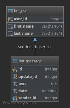
User
 model to hold the Telegram user-id and their names. Since we most certainly want to associate the messages we receive with the names of our registered users, let’s associate the user id with each message’s 
message['from']['id']
 field with the one from our 
User
 model to extract the user details like first- and last name from that; maybe we even add additional details to that table in the future, like an E-Mail- or postal address which then can be associated with each message of the same user-id. Adding a foreign key to our 
Message
 model is done using the ForeignKey field type like this:

class Message(models.Model):
    update_id       = models.IntegerField(unique=True)
    text            = models.TextField(max_length=4096)
    date            = models.DateTimeField(default=timezone.now)
    sender          = models.ForeignKey(User)

Also, we need to define what to do with each message if the user they are associated with is deleted from the table of our 

User
 model. We have a few choices here, predefined by how SQL works and explained in the “Arguments” section of the ForeignKey field type documentation. Let’s define that all messages which are associated with the deleted user record from the 
User
 model are deleted as well by changing the field definition to this:

class Message(models.Model):
    update_id       = models.IntegerField(unique=True)
    text            = models.TextField(max_length=4096)
    date            = models.DateTimeField(default=timezone.now)
    sender          = models.ForeignKey(User, on_delete=models.CASCADE)

Polishing and admin backend registration

Like we did with the 

User
 model already, let’s change the way the model’s elements are represented in the admin backend and register the model to the admin backend.

First, change the representation of our model to display our text by overwriting the definition for 

__str__
 like this:

class Message(models.Model):
    update_id       = models.IntegerField(unique=True)
    text            = models.TextField(max_length=4096)
    date            = models.DateTimeField(default=timezone.now)
    sender          = models.ForeignKey(User, on_delete=models.CASCADE)

    def __str__(self):
        return f'{self.text}'

This is our final form of that model definition so far, satisfying all our current needs.

Next, open the file 

bot/admin.py
 and make the following changes:
  1. Add 
    Message
     to the list of imports from 
    .models
     like this: 
    from .models import User, Message
  2. Add the line 
    admin.site.register(Message)
     to the file.

Now, save everything and let’s head for applying the migrations and double-check the results before with our final step for this article part we will do our deployment to production.

Creating and applying the migrations

Open up a shell, navigate and optionally active your virtualenv for your project and execute 

python manage.py makemigrations
 :

(dtbot-hT9CNosh) ~/dtbot $ python manage.py makemigrations
Migrations for 'bot':
  bot/migrations/0002_message.py
    - Create model Message
(dtbot-hT9CNosh) ~/dtbot $

Checking Git what this has caused shows that one migration file was created as desired, apart from which files we have changed manually before:

(dtbot-hT9CNosh) ~/dtbot $ git status -s
 M bot/admin.py
 M bot/models.py
?? bot/migrations/0002_message.py
(dtbot-hT9CNosh) ~/dtbot $

Let’s fire up 

migrate
 to have the migrations applied to our database:

(dtbot-hT9CNosh) ~/dtbot $ python manage.py migrate
Operations to perform:
  Apply all migrations: admin, auth, bot, contenttypes, sessions
Running migrations:
  Applying bot.0002_message... OK
(dtbot-hT9CNosh) ~/dtbot $

Our table fits into the SQL architecture like this:

Validating the results in the admin backend, you now should see that “Messages” shows in the “BOT” section and adding a record using the admin backend presents nice rendered fields to manipulate our data in a convenient way:

The date and time can be picked using convenient selectors, the up to 4096 characters long text is rendered as a Textarea instead a single-height input field and so on. What’s also pretty interesting: We can make selections for associating users we registered manually already – that might give you a nice idea that what we just tried to achieve does work like a charm! 👍

Deploy the changes to production

Using Heroku for our hosting, we have quite a few convenient tools at hands for our hosting. One of them is the ability to connect to our remote production database without needing to add any credentials or recognize names. While in your project folder, simply connect to your production database like this:

(dtbot-hT9CNosh) ~/dtbot $ heroku psql
--> Connecting to postgresql-rectangular-59399
psql (10.5 (Ubuntu 10.5-1.pgdg16.04+1))
SSL connection (protocol: TLSv1.2, cipher: ECDHE-RSA-AES256-GCM-SHA384, bits: 256, compression: off)
Type "help" for help.

dry-tundra-61874::DATABASE=> \dt
Did not find any relations.
dry-tundra-61874::DATABASE=> \q
(dtbot-hT9CNosh) ~/dtbot $

As we can see, there are no tables in our production database yet; fair, since we never applied any migrations to it. Let’s do this now for the first time.
Let’s first deploy our latest files by committing the changes to Git and push the commits to our Heroku remote, triggering a new deployment:

(dtbot-hT9CNosh) ~/dtbot $ git add .
(dtbot-hT9CNosh) ~/dtbot $ git commit -m "Adding a model for Messages"
[master a4de3de] Adding a model for Messages
 3 files changed, 39 insertions(+), 1 deletion(-)
 create mode 100644 bot/migrations/0002_message.py
(dtbot-hT9CNosh) ~/dtbot $ git push heroku master
Counting objects: 26, done.
Delta compression using up to 4 threads.
Compressing objects: 100% (25/25), done.
Writing objects: 100% (26/26), 6.11 KiB | 0 bytes/s, done.
Total 26 (delta 7), reused 0 (delta 0)
remote: Compressing source files... done.
remote: Building source:
remote: 
remote: -----> Python app detected
remote:        Using supported version of Python 3.6 (python-3.6.6)
remote: -----> Installing pip
remote: -----> Installing dependencies with Pipenv 2018.5.18…
remote:        Installing dependencies from Pipfile.lock (ce9952)…
remote: -----> $ python manage.py collectstatic --noinput
remote:        /app/.heroku/python/lib/python3.6/site-packages/psycopg2/__init__.py:144: UserWarning: The psycopg2 wheel package will be renamed from release 2.8; in order to keep installing from binary please use "pip install psycopg2-binary" instead. For details see: <http://initd.org/psycopg/docs/install.html#binary-install-from-pypi>.
remote:          """)
remote:        119 static files copied to '/tmp/build_751be55058319d19a3d47547d1362ed8/staticfiles', 362 post-processed.
remote: 
remote: -----> Discovering process types
remote:        Procfile declares types -> web
remote: 
remote: -----> Compressing...
remote:        Done: 65.3M
remote: -----> Launching...
remote:        Released v12
remote:        https://dry-tundra-61874.herokuapp.com/ deployed to Heroku
remote: 
remote: Verifying deploy... done.
To https://git.heroku.com/dry-tundra-61874.git
   2d16fea..a4de3de  master -> master
(dtbot-hT9CNosh) ~/dtbot $

That’s it! Our files are deployed, but still, that does not apply any migration to our database. Let’s do that as a final step for this part of the series.

Applying migrations to our production environment

Basically, you can execute any command you wish using the way I’m about to show you now; this time, we will apply our migrations to the production database. We will do that using a so-called “One-Off Dyno” with our Heroku account.
Unlike the regular dynos which are part of the dyno formation defined by the Procfile to operate our app’s regular business, One-Off Dynos do only have a limited life-span to execute specific administrative or maintenance tasks and are deleted upon logout again, leaving behind nothing but the permanent changes to the database or similar resources.

You are creating and logging in to them in one easy step:

(dtbot-hT9CNosh) ~/dtbot $ heroku run bash
Running bash on ⬢ dry-tundra-61874... up, run.1913 (Free)
~ $ hostname
0d532a3e-d79a-4314-9ad3-6e33f99f5b68
~ $ pwd
/app
~ $ ls -al
total 68
drwx------  7 u40905 dyno  4096 Nov  1 13:47 .
drwxr-xr-x 15 root   root  4096 Oct 29 15:35 ..
drwx------  4 u40905 dyno  4096 Nov  1 13:32 bot
drwx------  3 u40905 dyno  4096 Nov  1 13:32 dtbot
-rw-------  1 u40905 dyno    63 Nov  1 13:32 .gitignore
drwx------  4 u40905 dyno  4096 Nov  1 13:32 .heroku
-rwx------  1 u40905 dyno   537 Nov  1 13:32 manage.py
-rw-------  1 u40905 dyno   241 Nov  1 13:32 Pipfile
-rw-------  1 u40905 dyno 15659 Nov  1 13:32 Pipfile.lock
-rw-------  1 u40905 dyno    25 Nov  1 13:32 Procfile
drwx------  2 u40905 dyno  4096 Nov  1 13:32 .profile.d
-rw-------  1 u40905 dyno   291 Nov  1 13:32 requirements.txt
-rw-------  1 u40905 dyno    12 Nov  1 13:32 runtime.txt
drwx------  3 u40905 dyno  4096 Nov  1 13:32 staticfiles
~ $ python manage.py showmigrations
admin
 [ ] 0001_initial
 [ ] 0002_logentry_remove_auto_add
 [ ] 0003_logentry_add_action_flag_choices
auth
 [ ] 0001_initial
 [ ] 0002_alter_permission_name_max_length
 [ ] 0003_alter_user_email_max_length
 [ ] 0004_alter_user_username_opts
 [ ] 0005_alter_user_last_login_null
 [ ] 0006_require_contenttypes_0002
 [ ] 0007_alter_validators_add_error_messages
 [ ] 0008_alter_user_username_max_length
 [ ] 0009_alter_user_last_name_max_length
bot
 [ ] 0001_initial
 [ ] 0002_message
contenttypes
 [ ] 0001_initial
 [ ] 0002_remove_content_type_name
sessions
 [ ] 0001_initial
~ $

Awesome, isn’t it? We created and logged into a remote server-like environment, which only lives to fulfill a small task and after that will be deleted again with nothing left of it, without the need to care for login-security or doing anything manually. If we would logout of that now (Ctrl+d or typing “exit”, Enter), nothing would have changed; we only issued read operations. If your app would be operating in production already, this additional system would not affect it in any way. It would neither slow down your app by consuming resources like I/O or CPU, nor being unavailable for a few seconds or something for any reasons. If you would manipulate the database or destroy it, that would affect the production site for obvious reasons.
For now, imagine you just had the same database configured on a second instance of your code, just like you had these credentials entered into the local copy on your workstation.

Let’s initiate the database for Django, apply all outstanding migrations and create a superuser for it:

~ $ python manage.py migrate
Operations to perform:
  Apply all migrations: admin, auth, bot, contenttypes, sessions
Running migrations:
  Applying contenttypes.0001_initial... OK
  Applying auth.0001_initial... OK
  Applying admin.0001_initial... OK
  Applying admin.0002_logentry_remove_auto_add... OK
  Applying admin.0003_logentry_add_action_flag_choices... OK
  Applying contenttypes.0002_remove_content_type_name... OK
  Applying auth.0002_alter_permission_name_max_length... OK
  Applying auth.0003_alter_user_email_max_length... OK
  Applying auth.0004_alter_user_username_opts... OK
  Applying auth.0005_alter_user_last_login_null... OK
  Applying auth.0006_require_contenttypes_0002... OK
  Applying auth.0007_alter_validators_add_error_messages... OK
  Applying auth.0008_alter_user_username_max_length... OK
  Applying auth.0009_alter_user_last_name_max_length... OK
  Applying bot.0001_initial... OK
  Applying bot.0002_message... OK
  Applying sessions.0001_initial... OK
~ $ python manage.py createsuperuser
Username (leave blank to use 'u3090'): mrichter
Email address: foo@bar.de
Password: 
Password (again): 
Superuser created successfully.
~ $

Let’s see if that did anything to our database. Logout from that One-Off Dyno and reconnect to the remote PostgreSQL database 🐘:

~ $ exit
(dtbot-hT9CNosh) ~/dtbot $ heroku psql
--> Connecting to postgresql-rectangular-59399
psql (10.5 (Ubuntu 10.5-1.pgdg16.04+1))
SSL connection (protocol: TLSv1.2, cipher: ECDHE-RSA-AES256-GCM-SHA384, bits: 256, compression: off)
Type "help" for help.

dry-tundra-61874::DATABASE=> \dt
                      List of relations
 Schema |            Name            | Type  |     Owner      
--------+----------------------------+-------+----------------
 public | auth_group                 | table | gtdekhubrisukx
 public | auth_group_permissions     | table | gtdekhubrisukx
 public | auth_permission            | table | gtdekhubrisukx
 public | auth_user                  | table | gtdekhubrisukx
 public | auth_user_groups           | table | gtdekhubrisukx
 public | auth_user_user_permissions | table | gtdekhubrisukx
 public | bot_message                | table | gtdekhubrisukx
 public | bot_user                   | table | gtdekhubrisukx
 public | django_admin_log           | table | gtdekhubrisukx
 public | django_content_type        | table | gtdekhubrisukx
 public | django_migrations          | table | gtdekhubrisukx
 public | django_session             | table | gtdekhubrisukx
(12 rows)

dry-tundra-61874::DATABASE=>

BAAM; there they are: Our precious tables! 👊
This out of the way, nothing should prevent us from login into the admin backend using the credentials of the superuser we just created. As a shortcut: Execute 

heroku apps:open
 . That should spawn a browser and navigate it directly to your application’s site without the need to recognize anything.

Outlook for the next part of the series

You just learned how to craft models tailored for your use-case and how to deploy and apply these to your Heroku remote production environment. Also, you saw a few more handy heroku command-line client commands and learned how to make use of them for your development.

In the next article of this series, we will create a view which receives, filters and stores that messages in the database and a URLconf to expose that view, serving as an interface to provide to your Telegram bot as it’s webhook.
That means, that by the end of that part, our Telegram bot will be ready to be launched in production and already receive any amount of messages you and trustworthy users will send to it. 🤯

If you liked or disliked this article, I’d love to read that in the comments!

🐍 Enjoy coding! ❤

Born in 1982, Marc Richter is an IT enthusiastic since 1994. He became addicted when he first put hands on their family’s pc and never stopped investigating and exploring new things since then.
He is married to Jennifer Richter and proud father of two wonderful children, Lotta and Linus.
His current professional focus is DevOps and Python development.

An exhaustive bio can be found at this blog post.

Found my articles useful? Maybe you would like to support my efforts and give me a tip then?

Marc Richter's personal site - About Linux, programming in Python and Music

Made With Mu: Lesson Observation

$
0
0

I recently had the great pleasure of visiting Wollaston School to see Steve Foster use Mu in his classroom. Here he is in action, in perhaps the most “teacher-ish” photograph you’ll see for a long time:

This wasn’t my first visit to see Steve. He very kindly allowed me to observe his lessons back in 2017 when I was researching how learners and teachers engage with software development tools. His was the first of several schools and code clubs I visited for this purpose and, in addition to observing lessons, I interviewed him and some of his colleagues. In fact, it was as a direct result of chatting with the network administrators at Steve’s school that so much effort was put into making Mu easy to install. I was very pleased to hear that the very same network administrators had easily managed to install Mu on the computers in Steve’s classroom.

Achievement unlocked! :-)

On this visit I observed two lessons: a year 10 GCSE class (students turn 15 during year 10, and GCSE is the examination all students take at age 16), and a year 9 computing lesson (students turn 14 in year 9 and decide their “options” [which GCSE courses to take] during this academic year).

Both classes were exceptionally well behaved and engaged and the students were friendly and enthusiastic to learn. They’re a credit to themselves, Steve and their school.

I was simply introduced to the students as “Nicholas - a software developer” and played the role of a teaching assistant. This prompted a sense of nostalgia for me. Having students say, “Sir, I’m stuck on this problem” made me remember my time as a secondary head of music all those years ago and it was fun to collaborate with and support young people in their learning. There are some aspects of teaching which are extraordinarily rewarding and a privilege to experience – this was one such an occasion.

The students in year 10 knew what they were up to and were already familiar with Mu. It was good to see them use the editor with such fluency ~ to the extent that they were concentrating on their coding problem rather than getting side-tracked by their development environment. The first time I visited the school, I seem to remember students using some sort of online Python tool and I spent much of my time trying to help them fix the odd state into which they had got themselves. I also had a great sense of satisfaction when I saw how many of them were using the “Check” button to report potential problems with their code. They told me they found this especially useful when they ran their code and ended up with a syntax error. The “Check” button visually points out the problematic line and describes the problem. Far better than wading through terse computer-ese.

The year 9 class was especially enjoyable since I was watching their first encounter with Mu. In the previous academic year (before Mu 1.0 was released) they had been using IDLE as a development environment. Being able to observe their first contact with Mu was an amazing opportunity.

I wasn’t disappointed.

Steve started the lesson by introducing Mu as a new Python editor and then gave the class a few minutes to poke around with it before asking them to report back on what they’d discovered.

Within seconds, one of them had found the “Theme” button and toggled through to “night” mode. This was followed by a hilarious few seconds of excited whispering as the students all tried to turn their Mu editor into “night” mode. Within about a minute, everyone had “night” mode enabled and the class were feeling suitably “Hollywood hacker-ish”.

Some kids found the “Check” button while others enjoyed zooming in and out to extreme magnifications of their code. Most importantly, the feedback seemed positive and the students enjoyed playing with Mu (yes, “playing” is perhaps the right word).

Steve then asked them to “code along” a Magic 8 Ball script. Steve would explain some code and demonstrate it working, then ask the kids to type it in and check their version was working. After that, he’d repeatedly add more features, while giving the students an opportunity to ask questions, until the program was finished. This is exactly what Steve is doing in the photograph at the top of this blog post.

This activity was particularly fun since the students could define their own mysterious sounding Yes/No answers for the “magic 8 ball”. In a very teenager-y turn of events, one student cast their answers totally in the context of resolving relationship problems. Again, Mu didn’t cause any issues and the students could simply concentrate on customising their script.

At the end of both lessons I was given 10 minutes to tell the students a little bit about what I do as a software developer and enjoyed answering their questions. When Steve revealed I was the creator and maintainer of Mu, the year 9 class gave me a round of applause (after one girl started clapping loudly on her own, and then shouted to the rest of the class something along the lines of, “Give this guy some respect won’t ya..?”).

After the lessons Steve and I spent some time together in an interview / de-brief session. He provided more context about how Mu was used in his lessons and all the feedback I have received, be it from teacher or students, will find its way into improvements in the next version of Mu.

If you are a teacher using Mu in your classroom, please don’t hesitate to get in touch. We’d love to hear how you’re getting on and learn about the ways we can improve your own and your students’ experience of learning to program in Python.

Thanks to Steve and his students for giving me the rewarding experience of seeing Mu used in “real world” learning situations. Keep up the great work! :-)

Codementor: Decorators in python. What? Why? When?

$
0
0
A brief intro to python decorators and why they should be used.

Stack Abuse: Asynchronous Python for Web Development

$
0
0
Asynchronous Python for Web Development

Asynchronous programming is well suited for tasks that include reading and writing files frequently or sending data back and forth from a server. Asynchronous programs perform I/O operations in a non-blocking fashion, meaning that they can perform other tasks while waiting for data to return from a client rather than waiting idly, wasting resources and time.

Python, like many other languages, suffers from not being asynchronous by default. Fortunately, rapid changes in the IT world allow us to write asynchronous code even using languages that weren't originally meant to do so. Over the years, the demands for speed are exceeding hardware capabilities and companies around the world have come together with the Reactive Manifesto in order to deal with this issue.

The non-blocking behavior of asynchronous programs can result in significant performance benefits in the context of a web application, helping to address the issue of developing reactive apps.

Cooked into Python 3 are some powerful tools for writing asynchronous applications. In this article, we'll be covering some of these tools, especially as they relate to web development.

We'll be developing a simple reactive aiohttp based app to display the current relevant sky coordinates of planets from the Solar System, given the geographic coordinates of the user. You can find the app here, and the source code here.

We'll end up by discussing how to prepare the app to deploy to Heroku.

Introduction to Asynchronous Python

For those familiar with writing traditional Python code, making the jump to asynchronous code can be conceptually a little tricky. Asynchronous code in Python relies on coroutines, which in conjunction with an event loop allow for writing code that can appear to be doing more than one thing at a time.

Coroutines can be thought of as functions that have points in code where they give program control back to the calling context. These "yield" points allow for pausing and resuming coroutine execution, in addition to exchanging data between contexts.

The event loop decides what chunk of code runs at any given moment - it is responsible for pausing, resuming, and communicating between coroutines. This means that parts of different coroutines might end up executing in an order other than the one in which they were scheduled. This idea of running different chunks of code out of order is called concurrency.

Thinking about concurrency in the context of making HTTP requests can be elucidating. Imagine wanting to make many independent requests to a server. For example, we might want to query a website to get statistics about all the sports players in a given season.

We could make each request sequentially. However, with every request, we can imagine that out code might spend some time waiting around for a request to get delivered to the server, and for the response to be sent back.

Sometimes, these operations can take even multiple seconds. The application may experience network lag due to a high number of users, or simply due to the speed limits of the given server.

What if our code could do other things while waiting around for a response from the server? Moreover, what if it would only go back to processing a given request once response data arrived? We could make many requests in quick succession if we didn't have to wait for each individual request to finish before proceeding to the next in the list.

Coroutines with an event loop allow us to write code that behaves in exactly this manner.

asyncio

asyncio, part of the Python standard library, provides an event loop and a set of tools for controlling it. With asyncio we can schedule coroutines for execution, and create new coroutines (really asyncio.Task objects, using the parlance of asyncio) that will only finish executing once constituent coroutines finish executing.

Unlike other asynchronous programming languages, Python does not force us to use the event loop that ships with the language. As Brett Cannon points out, Python coroutines constitute an asynchronous API, with which we can use any event loop. Projects exist that implement a completely different event loop, like curio, or allow for dropping in a different event loop policy for asyncio (the event loop policy is what manages the event loop "behind the scenes"), like uvloop.

Let's take a look at a code snippet that runs two coroutines concurrently, each one printing out a message after one second:

# example1.py
import asyncio

async def wait_around(n, name):  
    for i in range(n):
        print(f"{name}: iteration {i}")
        await asyncio.sleep(1.0)

async def main():  
    await asyncio.gather(*[
        wait_around(2, "coroutine 0"), wait_around(5, "coroutine 1")
    ])

loop = asyncio.get_event_loop()  
loop.run_until_complete(main())  
me@local:~$ time python example1.py  
coroutine 1: iteration 0  
coroutine 0: iteration 0  
coroutine 1: iteration 1  
coroutine 0: iteration 1  
coroutine 1: iteration 2  
coroutine 1: iteration 3  
coroutine 1: iteration 4

real    0m5.138s  
user    0m0.111s  
sys     0m0.019s  

This code executes in roughly 5 seconds, as the asyncio.sleep coroutine establishes points at which the event loop can jump to executing other code. Moreover, we've told the event loop to schedule both wait_around instances for concurrent execution with the asyncio.gather function.

asyncio.gather takes a list of "awaitables" (ie, coroutines, or asyncio.Task objects) and returns a single asyncio.Task object that only finishes when all its constituent tasks/coroutines are finished. The last two lines are asyncio boilerplate for running a given coroutine until its finished executing.

Coroutines, unlike functions, won't start executing immediately after they're invoked. The await keyword is what tells the event loop to schedule a coroutine for execution.

If we take out the await in front of asyncio.sleep, the program finishes (almost) instantly, as we haven't told the event loop to actually execute the coroutine, which in this case tells the coroutine to pause for a set amount of time.

With a grasp of what asynchronous Python code looks like, let's move on to asynchronous web development.

Installing aiohttp

aiohttp is a Python library for making asynchronous HTTP requests. In addition, it provides a framework for putting together the server part of a web application. Using Python 3.5+ and pip, we can install aiohttp:

pip install --user aiohttp  

Client-Side: Making Requests

The following examples show how to we can download the HTML content of the "example.com" website using aiohttp:

# example2_basic_aiohttp_request.py
import asyncio  
import aiohttp

async def make_request():  
    url = "https://example.com"
    print(f"making request to {url}")
    async with aiohttp.ClientSession() as session:
        async with session.get(url) as resp:
            if resp.status == 200:
                print(await resp.text())

loop = asyncio.get_event_loop()  
loop.run_until_complete(make_request())  

A few things to emphasize:

  • Much like with await asyncio.sleep we must use await with resp.text() in order to get the HTML content of the page. If we left it out, our program's output would be something like the following:
me@local:~$ python example2_basic_aiohttp_request.py  
<coroutine object ClientResponse.text at 0x7fe64e574ba0>  
  • async with is a context manager that works with coroutines instead of functions. In both cases in which it gets used, we can imagine that internally, aiohttp is closing down connections to servers or otherwise freeing up resources.

  • aiohttp.ClientSession has methods that correspond to HTTP verbs. In the same way that session.get is making a GET request, session.post would make a POST request.

This example by itself offers no performance advantage over making synchronous HTTP requests. The real beauty of client-side aiohttp lies in making multiple concurrent requests:

# example3_multiple_aiohttp_request.py
import asyncio  
import aiohttp

async def make_request(session, req_n):  
    url = "https://example.com"
    print(f"making request {req_n} to {url}")
    async with session.get(url) as resp:
        if resp.status == 200:
            await resp.text()

async def main():  
    n_requests = 100
    async with aiohttp.ClientSession() as session:
        await asyncio.gather(
            *[make_request(session, i) for i in range(n_requests)]
        )

loop = asyncio.get_event_loop()  
loop.run_until_complete(main())  

Instead of making each request sequentially, we ask asyncio to do them concurrently, with asycio.gather.

PlanetTracker Web App

Through the course of this section, I intend to demonstrate how to put together an app that reports the current coordinates of planets in the sky at the user's location (ephemerides).

The user supplies his or her location with the web Geolocation API, which does the work for us.

I'll end up by showing how to set up a Procfile in order to deploy the app on Heroku. If you plan on following along as I work through putting the app together, you should do the following, assuming you have Python 3.6 and pip installed:

me@local:~$ mkdir planettracker && cd planettracker  
me@local:~/planettracker$ pip install --user pipenv  
me@local:~/planettracker$ pipenv --python=3  

Planet Ephemerides with PyEphem

An astronomical object's ephemeris is its current position in the sky at a given location and time on Earth. PyEphem is a Python library that allows for precisely calculating ephemerides.

It is especially well suited to the task at hand, as it has common astronomical objects cooked into the library. First, let's install PyEphem:

me@local:~/planettracker$ pipenv install ephem  

Getting the current coordinates of Mars is as simple as using an instance of the Observer class to compute its coordinates:

import ephem  
import math  
convert = math.pi / 180.  
mars = ephem.Mars()  
greenwich = ephem.Observer()  
greenwich.lat = "51.4769"  
greenwich.lon = "-0.0005"  
mars.compute(observer)  
az_deg, alt_deg = mars.az*convert, mars.alt*convert  
print(f"Mars' current azimuth and elevation: {az_deg:.2f} {alt_deg:.2f}")  

In order to make getting planet ephemerides easier, let's set up a class PlanetTracker with a method that returns a given planet's current azimith and altitude, in degrees (PyEphem defaults to using radians, not degrees, to represent angles internally):

# planet_tracker.py
import math  
import ephem

class PlanetTracker(ephem.Observer):

    def __init__(self):
        super(PlanetTracker, self).__init__()
        self.planets = {
            "mercury": ephem.Mercury(),
            "venus": ephem.Venus(),
            "mars": ephem.Mars(),
            "jupiter": ephem.Jupiter(),
            "saturn": ephem.Saturn(),
            "uranus": ephem.Uranus(),
            "neptune": ephem.Neptune()
        }

    def calc_planet(self, planet_name, when=None):
        convert = 180./math.pi
        if when is None:
            when = ephem.now()

        self.date = when
        if planet_name in self.planets:
            planet = self.planets[planet_name]
            planet.compute(self)
            return {
                "az": float(planet.az)*convert,
                "alt": float(planet.alt)*convert,
                "name": planet_name
            }
        else:
            raise KeyError(f"Couldn't find {planet_name} in planets dict")

Now we can get anyone of the seven other planets in the solar system quite easily:

from planet_tracker import PlanetTracker  
tracker = PlanetTracker()  
tracker.lat = "51.4769"  
tracker.lon = "-0.0005"  
tracker.calc_planet("mars")  

Running this piece of code would yield:

{'az': 92.90019644871396, 'alt': -23.146670983905302, 'name': 'mars'}

Server-Side aiohttp: HTTP Routes

Given some latitude and longitude, we can easily get a planet's current ephemeris, in degrees. Now let's set up an aiohttp route to allow a client to get a planet's ephemeris given the user's geolocation.

Before we can start writing code, we have to think about what HTTP verbs we want to associate with each of these tasks. It makes sense to use POST for the first task, as we're setting the observer's geographic coordinates. Given that we're getting ephemerides, it makes sense to use GET for the second task:

# aiohttp_app.py
from aiohttp import web

from planet_tracker import PlanetTracker


@routes.get("/planets/{name}")
async def get_planet_ephmeris(request):  
    planet_name = request.match_info['name']
    data = request.query
    try:
        geo_location_data = {
            "lon": str(data["lon"]),
            "lat": str(data["lat"]),
            "elevation": float(data["elevation"])
        }
    except KeyError as err:
        # default to Greenwich Observatory
        geo_location_data = {
            "lon": "-0.0005",
            "lat": "51.4769",
            "elevation": 0.0,
        }
    print(f"get_planet_ephmeris: {planet_name}, {geo_location_data}")
    tracker = PlanetTracker()
    tracker.lon = geo_location_data["lon"]
    tracker.lat = geo_location_data["lat"]
    tracker.elevation = geo_location_data["elevation"]
    planet_data = tracker.calc_planet(planet_name)
    return web.json_response(planet_data)


app = web.Application()  
app.add_routes(routes)

web.run_app(app, host="localhost", port=8000)  

Here, the route.get decorator indicates that we want the get_planet_ephmeris coroutine to be the handler for a variable GET route.

Before we run this, let's install aiohttp with pipenv:

me@local:~/planettracker$ pipenv install aiohttp  

Now we can run our app:

me@local:~/planettracker$ pipenv run python aiohttp_app.py  

When we run this, we can point our browser to our different routes to see the data our server returns. If I put localhost:8000/planets/mars into my browser's address bar, I should see some response like the following:

{"az": 98.72414165963292, "alt": -18.720718647020792, "name": "mars"}

This is the same as issuing the following curl command:

me@local:~$ curl localhost:8000/planets/mars  
{"az": 98.72414165963292, "alt": -18.720718647020792, "name": "mars"}

If you're not familiar with curl, it is a convenient command-line tool for, among other things, testing your HTTP routes.

We can supply a GET URL to curl:

me@local:~$ curl localhost:8000/planets/mars  
{"az": 98.72414165963292, "alt": -18.720718647020792, "name": "mars"}

This gives us Mars' ephemeris at the Greenwich Observatory in the UK.

We can encode coordinates in the URL of the GET request so we can get Mars' ephemeris at other locations (note the quotes around the URL):

me@local:~$ curl "localhost:8000/planets/mars?lon=145.051&lat=-39.754&elevation=0"  
{"az": 102.30273048280189, "alt": 11.690380174890928, "name": "mars"

curl can also be used to make POST requests as well:

me@local:~$ curl --header "Content-Type: application/x-www-form-urlencoded" --data "lat=48.93&lon=2.45&elevation=0" localhost:8000/geo_location  
{"lon": "2.45", "lat": "48.93", "elevation": 0.0}

Note that by providing the --data field, curl automatically assumes we're making a POST request.

Before we move on, I should note that the web.run_app function runs our app in a blocking manner. This is decidedly not what we're looking to accomplish!

To run it concurrently, we have to add a little more code:

# aiohttp_app.py
import asyncio  
...

# web.run_app(app)

async def start_app():  
    runner = web.AppRunner(app)
    await runner.setup()
    site = web.TCPSite(
        runner, parsed.host, parsed.port)
    await site.start()
    print(f"Serving up app on {parsed.host}:{parsed.port}")
    return runner, site

loop = asyncio.get_event_loop()  
runner, site = loop.run_until_complete(start_async_app())  
try:  
    loop.run_forever()
except KeyboardInterrupt as err:  
    loop.run_until_complete(runner.cleanup())

Note the presence of loop.run_forever instead of the call to loop.run_until_complete that we saw earlier. Instead of executing a set number of coroutines, we want our program to start a server that will handle requests until we exit with ctrl+c, at which point it will gracefully shutdown the server.

HTML/JavaScript Client

aiohttp allows us to serve up HTML and JavaScript files. Using aiohttp for serving "static" assets like CSS and JavaScript is discouraged, but for the purposes of this app, it shouldn't be an issue.

Let's add a few lines to our aiohttp_app.py file to serve up an HTML file that references a JavaScript file:

# aiohttp_app.py
...
@routes.get('/')
async def hello(request):  
    return web.FileResponse("./index.html")


app = web.Application()  
app.add_routes(routes)  
app.router.add_static("/", "./")  
...

The hello coroutine is setting up a GET route at localhost:8000/ that serves up the contents of index.html, located in the same directory from which we run our server.

The app.router.add_static line is setting up a route at localhost:8000/ to serve up files in the same directory from which we run our server. This means that our browser will be able to find the JavaScript file we reference in index.html.

Note: In production, it makes sense to move HTML, CSS and JS files into a separate directory that gets served up on its own. This makes it so the curious user cannot access our server code.

The HTML file is quite simple:

<!DOCTYPE html>  
<html lang='en'>

<head>  
    <meta charset="utf-8">
    <meta name="viewport" content="width=device-width, initial-scale=1">
    <title>Planet Tracker</title>
</head>  
<body>  
    <div id="app">
        <label id="lon">Longitude: <input type="text"/></label><br/>
        <label id="lat">Latitude: <input type="text"/></label><br/>
        <label id="elevation">Elevation: <input type="text"/></label><br/>
    </div>
    <script src="/app.js"></script>
</body>  

Though, the JavaScript file is a little more involved:

var App = function() {

    this.planetNames = [
        "mercury",
        "venus",
        "mars",
        "jupiter",
        "saturn",
        "uranus",
        "neptune"
    ]

    this.geoLocationIds = [
        "lon",
        "lat",
        "elevation"
    ]

    this.keyUpInterval = 500
    this.keyUpTimer = null
    this.planetDisplayCreated = false
    this.updateInterval = 2000 // update very second and a half
    this.updateTimer = null
    this.geoLocation = null

    this.init = function() {
        this.getGeoLocation().then((position) => {
            var coords = this.processCoordinates(position)
            this.geoLocation = coords
            this.initGeoLocationDisplay()
            this.updateGeoLocationDisplay()
            return this.getPlanetEphemerides()
        }).then((planetData) => {
            this.createPlanetDisplay()
            this.updatePlanetDisplay(planetData)
        }).then(() => {
            return this.initUpdateTimer()
        })
    }

    this.update = function() {
        if (this.planetDisplayCreated) {
            this.getPlanetEphemerides().then((planetData) => {
                this.updatePlanetDisplay(planetData)
            })
        }
    }

    this.get = function(url, data) {
        var request = new XMLHttpRequest()
        if (data !== undefined) {
            url += `?${data}`
        }
        // console.log(`get: ${url}`)
        request.open("GET", url, true)
        return new Promise((resolve, reject) => {
            request.send()
            request.onreadystatechange = function(){
                if (this.readyState === XMLHttpRequest.DONE && this.status === 200) {
                    resolve(this)
                }
            }
            request.onerror = reject
        })
    }

    this.processCoordinates = function(position) {
        var coordMap = {
            'longitude': 'lon',
            'latitude': 'lat',
            'altitude': 'elevation'
        }
        var coords = Object.keys(coordMap).reduce((obj, name) => {
            var coord = position.coords[name]
            if (coord === null || isNaN(coord)) {
                coord = 0.0
            }
            obj[coordMap[name]] = coord
            return obj
        }, {})
        return coords
    }

    this.coordDataUrl = function (coords) {
        postUrl = Object.keys(coords).map((c) => {
            return `${c}=${coords[c]}`
        })
        return postUrl
    }

    this.getGeoLocation = function() {
        return new Promise((resolve, reject) => {
            navigator.geolocation.getCurrentPosition(resolve)
        })
    }

    this.getPlanetEphemeris = function(planetName) {
        var postUrlArr = this.coordDataUrl(this.geoLocation)
        return this.get(`/planets/${planetName}`, postUrlArr.join("&")).then((req) => {
            return JSON.parse(req.response)
        })
    }

    this.getPlanetEphemerides = function() {
        return Promise.all(
            this.planetNames.map((name) => {
                return this.getPlanetEphemeris(name)
            })
        )
    }

    this.createPlanetDisplay = function() {
        var div = document.getElementById("app")
        var table = document.createElement("table")
        var header = document.createElement("tr")
        var headerNames = ["Name", "Azimuth", "Altitude"]
        headerNames.forEach((headerName) => {
            var headerElement = document.createElement("th")
            headerElement.textContent = headerName
            header.appendChild(headerElement)
        })
        table.appendChild(header)
        this.planetNames.forEach((name) => {
            var planetRow = document.createElement("tr")
            headerNames.forEach((headerName) => {
                planetRow.appendChild(
                    document.createElement("td")
                )
            })
            planetRow.setAttribute("id", name)
            table.appendChild(planetRow)
        })
        div.appendChild(table)
        this.planetDisplayCreated = true
    }

    this.updatePlanetDisplay = function(planetData) {
        planetData.forEach((d) => {
            var content = [d.name, d.az, d.alt]
            var planetRow = document.getElementById(d.name)
            planetRow.childNodes.forEach((node, idx) => {
                var contentFloat = parseFloat(content[idx])
                if (isNaN(contentFloat)) {
                    node.textContent = content[idx]
                } else {
                    node.textContent = contentFloat.toFixed(2)
                }
            })
        })
    }

    this.initGeoLocationDisplay = function() {
        this.geoLocationIds.forEach((id) => {
            var node = document.getElementById(id)
            node.childNodes[1].onkeyup = this.onGeoLocationKeyUp()
        })
        var appNode = document.getElementById("app")
        var resetLocationButton = document.createElement("button")
        resetLocationButton.setAttribute("id", "reset-location")
        resetLocationButton.onclick = this.onResetLocationClick()
        resetLocationButton.textContent = "Reset Geo Location"
        appNode.appendChild(resetLocationButton)
    }

    this.updateGeoLocationDisplay = function() {
        Object.keys(this.geoLocation).forEach((id) => {
            var node = document.getElementById(id)
            node.childNodes[1].value = parseFloat(
                this.geoLocation[id]
            ).toFixed(2)
        })
    }

    this.getDisplayedGeoLocation = function() {
        var displayedGeoLocation = this.geoLocationIds.reduce((val, id) => {
            var node = document.getElementById(id)
            var nodeVal = parseFloat(node.childNodes[1].value)
            val[id] = nodeVal
            if (isNaN(nodeVal)) {
                val.valid = false
            }
            return val
        }, {valid: true})
        return displayedGeoLocation
    }

    this.onGeoLocationKeyUp = function() {
        return (evt) => {
            // console.log(evt.key, evt.code)
            var currentTime = new Date()
            if (this.keyUpTimer !== null){
                clearTimeout(this.keyUpTimer)
            }
            this.keyUpTimer = setTimeout(() => {
                var displayedGeoLocation = this.getDisplayedGeoLocation()
                if (displayedGeoLocation.valid) {
                    delete displayedGeoLocation.valid
                    this.geoLocation = displayedGeoLocation
                    console.log("Using user supplied geo location")
                }
            }, this.keyUpInterval)
        }
    }

    this.onResetLocationClick = function() {
        return (evt) => {
            console.log("Geo location reset clicked")
            this.getGeoLocation().then((coords) => {
                this.geoLocation = this.processCoordinates(coords)
                this.updateGeoLocationDisplay()
            })
        }
    }

    this.initUpdateTimer = function () {
        if (this.updateTimer !== null) {
            clearInterval(this.updateTimer)
        }
        this.updateTimer = setInterval(
            this.update.bind(this),
            this.updateInterval
        )
        return this.updateTimer
    }

    this.testPerformance = function(n) {
        var t0 = performance.now()
        var promises = []
        for (var i=0; i<n; i++) {
            promises.push(this.getPlanetEphemeris("mars"))
        }
        Promise.all(promises).then(() => {
            var delta = (performance.now() - t0)/1000
            console.log(`Took ${delta.toFixed(4)} seconds to do ${n} requests`)
        })
    }
}

var app  
document.addEventListener("DOMContentLoaded", (evt) => {  
    app = new App()
    app.init()
})

This app will periodically (every 2 seconds) update and display planet ephemerides. We can supply our own geo coordinates, or let the Web Geolocation API determine our current location. The app updates the geolocation if the user stops typing for a half a second or more.

While this is not a JavaScript tutorial, I think it's useful to understand what different parts of the script are doing:

  • createPlanetDisplay is dynamically creating HTML elements and binding them to the Document Object Model (DOM)
  • updatePlanetDisplay takes data received from the server and populates the elements created by createPlanetDisplay
  • get makes a GET request to the server. The XMLHttpRequest object allows this to be done without reloading the page.
  • post makes a POST request to the server. Like with get this is done without reloading the page.
  • getGeoLocation uses the Web Geolocation API to get the user's current geographic coordinates. This must be fulfilled "in a secure context" (ie we must be using HTTPSnotHTTP).
  • getPlanetEphemeris and getPlanetEphemerides make GET requests to the server to get ephemeris for a specific planet and to get ephemerides for all planets, respectively.
  • testPerformance makes n requests to the server, and determines how long it takes.

Primer on Deploying to Heroku

Heroku is a service for easily deploying web applications. Heroku takes care of configuring web-facing components of an application, like configuring reverse proxies or worrying about load balancing. For applications handling few requests and a small number of users, Heroku is a great free hosting service.

Deploying Python applications to Heroku has become very easy in recent years. At its core, we have to create two files that list our application's dependencies and tell Heroku how to run our application.

A Pipfile takes care of the former, while a Procfile takes care of the latter. A Pipfile is maintained by using pipenv - we add to our Pipfile (and Pipfile.lock) every time we install a dependency.

In order to run our app on Heroku, we have to add one more dependency:

me@local:~/planettracker$ pipenv install gunicorn  

We can create our own Procfile, adding the following line to it:

web: gunicorn aiohttp_app:app --worker-class aiohttp.GunicornWebWorker  

Basically this is telling Heroku to use Gunicorn to run our app, using the special aiohttp web worker.

Before you can deploy to Heroku, you'll need to start tracking the app with Git:

me@local:~/planettracker$ git init  
me@local:~/planettracker$ git add .  
me@local:~/planettracker$ git commit -m "first commit"

Now you can follow the instructions on the Heroku devcenter here for deploying your app. Note that you can skip the "Prepare the App" step of this tutorial, as you already have a git tracked app.

Once your application is deployed, you can navigate to the chosen Heroku URL in your browser and view the app, which will look something like this:

Asynchronous Python for Web Development

Conclusion

In this article, we dived into what asynchronous web development in Python looks like - it's advantages and uses. Afterwards, we built a simple reactive aiohttp based app that dynamically displays the current relevant sky coordinates of planets from the Solar System, given the geographic coordinates of the user.

Upon building the application, we've prepped it for deployment on Heroku.

As mentioned before, you can find both the source code and application demo if needed.

Full Stack Python: Adding Okta Authentication to an Existing Flask Web App

$
0
0

It can be a lot of work to piece together a full authentication system if you have an existing Flask web application that you are coding. Okta makes it much easier to drop-in a complete user authentication system without a lot of additional effort. In this tutorial we will take the Flask Git Dashboard project as an example and add Okta to it.

Libraries

Python 3 is required for this tutorial and we will also use:

All of the finished code in this blog post is provided as open source under the MIT license on GitHub under the auth-existing-flask-app/finished directory of the blog-code-examples repository. Use and abuse the source code for your own applications.

Installing Dependencies

We will start out with an existing Flask web application. If you do not have your own that you are modifying, clone this Git repository:

git clone git@github.com:fullstackpython/blog-code-examples.git

Next, create a new Python virtualenv for this project:

python3 -m venv flaskauth

Activate the virtual environment with the activate script:

. ./flaskauth/bin/activate

The command prompt should change after activation:

Activating the flaskauth virtualenv.

Remember that you will have to activate the virtualenv in every terminal window where you want to use the dependencies contained in this virtualenv.

Change into the project directory within the block-code-examples Git repository that you cloned.

cd blog-code-examples/auth-existing-flask-app/start/

Now we can install the dependencies for the existing project.

pip install -r requirements.txt

Look for output similar to the following to confirm that the dependencies successfully installed:

...
Collecting amqp<3.0,>=2.1.4 (from kombu<5.0,>=4.0.2->Celery==4.1.0->-r requirements.txt (line 4))
  Downloading https://files.pythonhosted.org/packages/7f/cf/12d4611fc67babd4ae250c9e8249c5650ae1933395488e9e7e3562b4ff24/amqp-2.3.2-py2.py3-none-any.whl (48kB)
    100% |████████████████████████████████| 51kB 10.7MB/s 
Collecting six>=1.5 (from python-dateutil->alembic>=0.6->Flask-Migrate==2.2.0->-r requirements.txt (line 2))
  Using cached https://files.pythonhosted.org/packages/67/4b/141a581104b1f6397bfa78ac9d43d8ad29a7ca43ea90a2d863fe3056e86a/six-1.11.0-py2.py3-none-any.whl
Collecting vine>=1.1.3 (from amqp<3.0,>=2.1.4->kombu<5.0,>=4.0.2->Celery==4.1.0->-r requirements.txt (line 4))
  Downloading https://files.pythonhosted.org/packages/10/50/5b1ebe42843c19f35edb15022ecae339fbec6db5b241a7a13c924dabf2a3/vine-1.1.4-py2.py3-none-any.whl
Installing collected packages: click, itsdangerous, Werkzeug, MarkupSafe, Jinja2, Flask, SQLAlchemy, Flask-SQLAlchemy, Mako, python-editor, six, python-dateutil, alembic, Flask-Migrate, billiard, pytz, vine, amqp, kombu, Celery, redis, WTForms
  Running setup.py install for MarkupSafe ... done
  Running setup.py install for SQLAlchemy ... done
  Running setup.py install for Mako ... done
  Running setup.py install for python-editor ... done
  Running setup.py install for alembic ... done
  Running setup.py install for billiard ... done
  Running setup.py install for WTForms ... done
Successfully installed Celery-4.1.0 Flask-1.0.2 Flask-Migrate-2.2.0 Flask-SQLAlchemy-2.3.2 Jinja2-2.10 Mako-1.0.7 MarkupSafe-1.0 SQLAlchemy-1.2.12 WTForms-2.1 Werkzeug-0.14.1 alembic-1.0.1 amqp-2.3.2 billiard-3.5.0.4 click-7.0 itsdangerous-1.1.0 kombu-4.2.1 python-dateutil-2.7.5 python-editor-1.0.3 pytz-2018.7 redis-2.10.6 six-1.11.0 vine-1.1.4

We need a couple of additional dependencies for our project to work, flask-oidc and okta:

pip install flask-oidc>=1.4.0 okta==0.0.4

The dependencies are now properly installed into our virtual environment. Let's test out the application to see if we can get it running properly.

export FLASK_APP=flaskdash.py
export FLASK_ENV=development
flask run

We should see the application start up with some default development time values:

 * Serving Flask app "flaskdash.py"(lazy loading)
 * Environment: development
 * Debug mode: on
 * Running on http://127.0.0.1:5000/ (Press CTRL+C to quit)
 * Restarting with stat
 * Debugger is active!
 * Debugger PIN: 203-814-092

Head to localhost:5000 in your web browser and we should see a work-in-progress dashboard:

Dashboard provided by existing Flask application.

It's time to get to setting up an Okta developer account so we can get the appropriate configuration information for our application.

Okta for Authentication

Head to the Okta developers sign up page.

Okta developers landing page for signing up.

Sign up for a new account or log into your existing account.

Okta developer sign up flow.

The interesting bit about the Okta developer sign up flow is that now you should check your email to finish creating your account. Look for an email like this one:

Okta sign up email.

Click the "Sign In" button and log into developer account using the temporary password found in the email. Set a new password and challenge question. Then pick an image to match your account login process.

Okta finish creating an account.

Click the "Create Account" button and you will be wisked away to the Okta developer dashboard.

Okta developer dashboard.

Find the "Org URL" as shown in the following image.

Okta Org URL value.

We are going to use that URL in our secret credentials file so that our Flask web app can properly connect to the Okta service.

Create a new file in your project directory named openidconnect_secrets.json with the following contents:

{"web":{"client_id":"{{ OKTA_CLIENT_ID }}","client_secret":"{{ OKTA_CLIENT_SECRET }}","auth_uri":"{{ OKTA_ORG_URL }}/oauth2/default/v1/authorize","token_uri":"{{ OKTA_ORG_URL }}/oauth2/default/v1/token","issuer":"{{ OKTA_ORG_URL }}/oauth2/default","userinfo_uri":"{{ OKTA_ORG_URL }}/oauth2/default/userinfo","redirect_uris":["http://localhost:5000/oidc/callback"]}}

Replace the four {{ OKTA_ORG_URL }} placeholders with the Org URL value found in your dashboard. We will fill in the rest of the placeholders with actual values as we proceed through the tutorial. My openidconnect_secret.json file would currently have the following values based on my developer dashboard Org URL. Remember that your URL values will be different!

{"web":{"client_id":"{{ OKTA_CLIENT_ID }}","client_secret":"{{ OKTA_CLIENT_SECRET }}",~~"auth_uri":"https://dev-860408.oktapreview.com/oauth2/default/v1/authorize",~~"token_uri":"https://dev-860408.oktapreview.com/oauth2/default/v1/token",~~"issuer":"https://dev-860408.oktapreview.com/oauth2/default",~~"userinfo_uri":"https://dev-860408.oktapreview.com/oauth2/default/userinfo","redirect_uris":["http://localhost:5000/oidc/callback"]}}

Okay awesome, we have our Okta account set up so we can add the authentication code to our Flask application.

Updating the Flask App with Okta

We need to connect our Flask code to our new Okta account. The recommended way of including variables such as account credentials in a Flask application is through configuration handling.

Update config.py the Flask code with the following highlighted lines.

importosclassConfig(object):SECRET_KEY=os.getenv('SECRET_KEY')or'development key'# RedisREDIS_SERVER=os.getenv('REDIS_SERVER')or'localhost'REDIS_PORT=os.getenv('REDIS_PORT')or6379REDIS_DB=os.getenv('REDIS_DB')or1REDIS_URL='redis://{}:{}'.format(REDIS_SERVER,REDIS_PORT)# Celery task queueCELERY_BROKER_URL=os.getenv('CELERY_BROKER_URL')orREDIS_URLCELERY_RESULT_BACKEND=os.getenv('CELERY_RESULT_BACKEND')orREDIS_URL# database settingsSQLALCHEMY_DATABASE_URI=os.getenv('DATABASE_URL')or \
      'sqlite:///'+os.path.join(os.path.abspath(os.path.dirname(__file__)),'flaskdash.db')SQLALCHEMY_TRACK_MODIFICATIONS=False~~~~OIDC_CLIENT_SECRETS="openidconnect_secrets.json"~~OIDC_COOKIE_SECURE=False~~OIDC_CALLBACK_ROUTE="/oidc/callback"~~OIDC_SCOPES=["openid","email","profile"]~~OIDC_ID_TOKEN_COOKIE_NAME="oidc_token"

We first add three import lines, one to pull values from environment variables, and the next two imports to make it possible to use OpenID Connect and Okta in our application.

The rest of the new code sets Flask application configuration values that can be used to instantiate the OpenID Connect and Okta clients.

  • OIDC_CLIENT_SECRETS: the location of the OpenID Connect secrets file
  • OIDC_COOKIE_SECURE: allows development mode for testing user login and registration without SSL. Your application must set this to True in a production application.
  • OIDC_CALLBACK_ROUTE: URL in the web app for handling user logins
  • OIDC_SCOPES: what data to request about the user when they log in. Our application requests the basic email, name and profile information
  • SECRET_KEY: this is a Flask setting to keep sessions secure. The key must never be made public or your web application user sessions will be compromised.

Where do we get those application configuration values though? We need to obtain them from our Okta account so go back to the dashboard to create a new OpenID Connect application.

Select applications on the Okta developer dashboard.

OpenID Connect applications use a client ID and client secret in place of traditional usernames and passwords. The client ID and client secret will tell your authorization server to recognize your application. Press the "Add Application" button.

Click the Add Application button.

On the new application screen choose "Web" and then press "Next".

Choose a web application.

On the next page there are numerous configuration options but only a few values we need to fill in before we can get our credentials. Set the following values to the Name, Base URIs and Login redirect URIs properties:

  1. FlaskApp for Name
  2. http://localhost:5000 for Base URIs
  3. http://localhost:5000/oidc/callback for Login redirect URIs

Set application configuration values.

Those are the three values you need to fill in for now so save the application to create it.

On the next page scroll down to find your client and secret keys.

Save the client credentials for later use.

Copy and paste the client ID and client secret into the following highlighted lines to replace the {{ OKTA_CLIENT_ID }} and {{ OKTA_CLIENT_SECRET }} placeholders.

{"web":{~~"client_id":"{{ OKTA_CLIENT_ID }}",~~"client_secret":"{{ OKTA_CLIENT_SECRET }}","auth_uri":"https://dev-860408.oktapreview.com/oauth2/default/v1/authorize","token_uri":"https://dev-860408.oktapreview.com/oauth2/default/v1/token","issuer":"https://dev-860408.oktapreview.com/oauth2/default","userinfo_uri":"https://dev-860408.oktapreview.com/oauth2/default/userinfo","redirect_uris":["http://localhost:5000/oidc/callback"]}}

Save the file and make sure to keep it out of version control as those secret values need to stay secret.

We have one more step in the Okta developer dashboard before we upgrade our Flask application with the authentication code: creating an API authentication token. Go to the API tab.

Click the API tab in the dashboard.

Click the "Create Token" button.

Create an authentication token to access Okta.

Name the token FlaskToken and copy it. Save the token somewhere safe as we will not be able to access it through the dashboard again. We are going to use this token when setting the OKTA_AUTH_TOKEN environment variable in the next section of this tutorial.

Okay, we finally have all the Okta service configuration and tokens in our openidconnect_secret.json file that we need to finish our application.

Update app/__init__.py with these highlighted lines:

importredis~~fromosimportenvironfromflaskimportFlaskfromapp.utilsimportmake_celeryfromconfigimportConfigfromflask_sqlalchemyimportSQLAlchemyfromflask_migrateimportMigrate~~fromflask_oidcimportOpenIDConnect~~fromoktaimportUsersClientapp=Flask(__name__,static_url_path='/static')app.config.from_object(Config)db=SQLAlchemy(app)migrate=Migrate(app,db)# connect to Redis instanceredis_db=redis.StrictRedis(host=app.config['REDIS_SERVER'],port=app.config['REDIS_PORT'],db=app.config['REDIS_DB'])celery=make_celery(app)~~# instantiate OpenID client to handle user session~~oidc=OpenIDConnect(app)~~# Okta client will determine if a user has an appropriate account~~okta_client=UsersClient(environ.get("OKTA_ORG_URL"),~~environ.get("OKTA_AUTH_TOKEN"))fromappimportroutes

We can now access the okta_client in our routes. Open app/routes.py and update the following lines:

fromflaskimportsend_from_directory,render_templatefromflaskimportredirect,g~~fromappimportapp,oidc,okta_client~~@app.before_request~~defbefore_request():~~ifoidc.user_loggedin:~~g.user=okta_client.get_user(oidc.user_getfield("sub"))~~else:~~g.user=None@app.route('/js/<path:path>')defsend_js(path):returnsend_from_directory('js',path)@app.route('/css/<path:path>')defsend_css(path):returnsend_from_directory('css',path)@app.route("/")defdashboard():returnrender_template('dashboard.html')@app.route("/repositories")~~@oidc.require_logindefrepositories():returnrender_template('repositories.html')~~@app.route("/login")~~@oidc.require_login~~deflogin():~~returnredirect(url_for(".repositories"))~~~~~~@app.route("/logout")~~deflogout():~~oidc.logout()~~returnredirect(url_for(".landing_page"))

The above new highlighted lines check whether or not a user is logged in before each request. If a route requires a logged in user due to the @oidc.require_login decorator then the user will be redirect to the sign in page. We also added routes under /login and /logout to make it possible to log in and out of the application.

Set three environment variables so our application can use them when we run it. Make sure the placeholders ORG_URL and AUTH_TOKEN are set with your actual Org URL value and auth token from the Okta developer dashboard.

On the command line run the following commands, making sure to replace any placeholder values with your own tokens and URLs:

# this tells Flask we want to run the built-in server in dev mode
export FLASK_ENV=development
# make sure to use a very long random string here that cannot be guessed
export SECRET_KEY='a very long string with lots of numbers and letters'
# this is the same Org URL found on your developer dashboard
# for example, https://dev-860408.oktapreview.com
export OKTA_ORG_URL='ORG_URL'
# this is the API authentication token we created
export OKTA_AUTH_TOKEN='AUTH_TOKEN'

Now re-run the Flask application:

set FLASK_APP=app.py
flask run

You should be in good shape if the development server starts up with output like this:

(flaskauth)$ flask run
 * Environment: development
 * Debug mode: on
 * Running on http://127.0.0.1:5000/ (Press CTRL+C to quit)
 * Restarting with stat
 * Debugger is active!
 * Debugger PIN: 415-920-546

Head to localhost:5000 in a browser where you are not already logged into your Okta account (an incognito window of your web browser works great).

Dashboard while in incognito mode.

Let's test the redirect functionality when we try to go to the /dashboard route by going to localhost:5000/repositories. We get redirected to the Okta login page.

Getting redirected while in incognito mode.

Enter your Okta developer username and password to log into your application. For development purposes this will work fine for testing but obviously in a production application you will create other accounts for users to log into.

Got into the repositories page after logging in.

To unauthenticate your user go to localhost:5000/logout. When you go back to localhost:5000/repositories again you will now have to re-authenticate.

What Now?

We configured an existing Flask application to use Okta for user authentication and identity management via the Okta API.

Next you can try one of the following tutorials to add other features to the Flask application:

You can also determine what to code next in your Python project by reading the Full Stack Python table of contents page.

Questions? Contact me via Twitter @fullstackpython or @mattmakai. I am also on GitHub with the username mattmakai.

Something wrong with this post? Fork this page's source on GitHub and submit a pull request.

Viewing all 22646 articles
Browse latest View live


<script src="https://jsc.adskeeper.com/r/s/rssing.com.1596347.js" async> </script>