Quantcast
Channel: Planet Python
Viewing all 22647 articles
Browse latest View live

Bill Ward / AdminTome: Python Set: Tutorial for Python Beginners

$
0
0

In this post I will go over what a Python set is and how to use them in your Python programs. With sets we can manage data just like math sets.

Python sets let us work with sets of values much like we do in math.

Video Tutorial

Creating a Set

You create a set using the curly brackets:  {}  much like when you declare a dictionary.

The difference is that sets don’t have a key value like dictionaries do.

For example, we will create a set with numbers from 0 to 3:

mySet = {0, 1, 2, 3}

Sets have unique values.  So if you declare a set with duplicate values, you will end up with a set that only contains the unique values:

In [1]: mySet = {1,2,3,4}

In [2]: mySet
Out[2]: {1, 2, 3, 4}

In [3]: badSet = {1,1,2,3}

In [4]: badSet
Out[4]: {1, 2, 3}

In [5]: 

As you can see, when I initialized badSet it had duplicate values (the number 1 was listed twice) but when I show the value of the set it only showed the unique values 1, 2, and 3.

We can even create sets from Strings.

In [8]: nameSet = {"Bob", "Frank", "Jill", "Jack"}

In [9]: nameSet
Out[9]: {'Bob', 'Frank', 'Jack', 'Jill'}

Set Ordering

One thing to note is that the ordering of the values is not important.

In [7]: mySet
Out[7]: {1, 2, 3, 6, 8, 10}

This works for strings as well as you may have noticed from the nameSet example above.

In [8]: nameSet = {"Bob", "Frank", "Jill", "Jack"}

In [9]: nameSet
Out[9]: {'Bob', 'Frank', 'Jack', 'Jill'}

Just because the Python set displays the list ordered doesn’t mean if you iterate over it you will get the ordering.

In [11]: for name in nameSet:
    ...:     print("Student: {}".format(name))
    ...:     
Student: Frank
Student: Bob
Student: Jill
Student: Jack

This is because with sets we only care that the value exists and nothing else.

Converting other data types

We can convert other data types to a set using  set() .

For example, we can convert a list to a set.

In [14]: myList = ["Paladin","Roque","Warrior"]

In [15]: mySet = set(myList)

In [16]: mySet
Out[16]: {'Paladin', 'Roque', 'Warrior'}

or a dictionary:

In [17]: myDict = {"class": "Paladin", "name": "Belkas", "server": "Malfurion"}

In [18]: mySet = set(myDict)

In [19]: mySet
Out[19]: {'class', 'name', 'server'}

Notice that the our Python set only contains the key values of our dictionary.

Set Theory

In this section, we use sets like we learned in math class.

Python Set Theory

In this section we are going to use these sets.

In [27]: primeNums = {1, 2, 3, 5, 7, 11, 13, 17, 19}

In [28]: myNums = set(range(20))

In [29]: myNums
Out[29]: {0, 1, 2, 3, 4, 5, 6, 7, 8, 9, 10, 11, 12, 13, 14, 15, 16, 17, 18, 19}

We can combine sets in several ways.

We can see what values exists in both sets using the ampersand ‘&’ operator.  This is called the intersection of the two sets.

In [30]: primeNums & myNums
Out[30]: {1, 2, 3, 5, 7, 11, 13, 17, 19}

We can see what values that exist in either set called the union of the two sets using the bar ‘|’ or the union() python function.

In [31]: primeNums | myNums
Out[31]: {0, 1, 2, 3, 4, 5, 6, 7, 8, 9, 10, 11, 12, 13, 14, 15, 16, 17, 18, 19}

In [32]: primeNums.union(myNums)
Out[32]: {0, 1, 2, 3, 4, 5, 6, 7, 8, 9, 10, 11, 12, 13, 14, 15, 16, 17, 18, 19}

We can see what values exist in the first set but don’t exist in the second set with the difference operator ‘-‘

In [33]: primeNums - myNums
Out[33]: set()

This gives us an empty set because all the values in primeNums exists in myNums.  Lets turn it around.

In [36]: myNums - primeNums
Out[36]: {0, 4, 6, 8, 9, 10, 12, 14, 15, 16, 18}

This gives us a set of numbers from myNums that are not prime numbers.

Conclusion

There is more to Python sets but I covered the basics here to get you started.  For more information checkout the Python Reference.

Be sure to checkout other great Python articles on AdminTome Blog.

If you liked this post then please share it and comment below.  I would love to hear from you.

The post Python Set: Tutorial for Python Beginners appeared first on AdminTome Blog.


Codementor: Essential Tips and Tricks for Starting Machine Learning with Python

$
0
0
We describe some essential hacks and tricks for practicing machine learning with Python. Covers most important libraries, and the overall approach.

Mike Driscoll: PyDev of the Week: Thea Flowers

$
0
0

This week we welcome Thea Flowers (@theavalkyrie) as our PyDev of the Week! Thea is a maintainer of packaging.python.org and the urllib3 package. Thea also is very active in the Python community and is a new board member of the Python Software Foundation. You can find out more about Thea on her website, Github. Let’s take a few moments to get to know Thea better!

Can you tell us a little about yourself (hobbies, education, etc):

I’m currently at Google where I work in Developer Relations for Google Cloud Platform. I focus on API client libraries and supporting the Python community. I even have the official title of “Pythonista”! I’m also the co-chair for PyCascades 2019 which will take place in Seattle early next year. Outside of professional commitments, I like to build synthesizers and costume props and I also volunteer as a mentor for FIRST Robotics.

I have a pretty non-traditional background. I’m originally from Atlanta, Georgia and I have no higher education to speak of. I worked by way into being a professional software engineer via open source and a lot of luck. I started programming as a teenager to attempt to make video games. I never managed to make a video game but I had a lot of fun trying and learned a ton of useful skills.

Oh, I’m also openly transgender.

Why did you start using Python?

I believe the first time I used Python was when I was a teenager. I was building a 2D game engine using C++ and wanted a continuous build system. Of course, I had no idea that the term even existed, but I decided to throw together something that could automatically build the engine every time I committed to SVN. I believe I built it with CherryPy and Cheetah templates.

What other programming languages do you know and which is your favorite?

I work a lot in C/C++ (for programming Arduino-based projects and previously when making game engines) as well as lots of JavaScript and occasionally some Go. I’ve worked in a lot of other languages as well. Python is above and beyond my favorite. I often find myself using it even when programming in other languages. For example, I used Python recently to experiment with a parser for a synthesizer patch format before porting it to C++.

What projects are you working on now?

At Google I’m currently working on automating a lot of our process of generating and publishing client libraries. I’m building tools that can run and combine the output of several code generators (think protobuf/swagger/openapi) and create a working library. All of this automation is written in Python.

Outside of Google I’m working on building a hardware synthesizer based on the YM2612, the sound chip used in the Sega Genesis (or MegaDrive). You can read more about that here or follow along on Twitter.

I also have a collection of Open Source projects that I’m involved in: Urllib3, Nox, packaging.python.org, readme_renderer, cmarkgfm, etc.

Which Python libraries are your favorite (core or 3rd party)?

Too many to enumerate. I was recently chatting with a coworker about how amazing and useful the core struct module is. I use it all the time for getting Python programs to chat with other hardware over serial and parsing binary file formats.

What challenges did you face and overcome when working on the packaging.python.org site?

The biggest challenge with a project that is that visible is consensus. Getting all of the people who care about something to agree how to do something is often really hard. Being able to drive consensus is a really critical skill for someone who wants to really own an open source project. That said, for the most part things have gone really smoothly with that project. I still think we have so much more to do there but it’s getting better all the time.

Do you have any tips for people who would like to contribute to one of your projects?

Look for the “contributor friendly” or “for first timer” labels and start commenting and asking questions. Also, always feel free to reach out to me. I’m always happy to do a video chat or pair programming session to help people get their first contribution in.

How do you keep your volunteers motivated in open source?

One of the biggest things I feel a primary maintainer can do is remove ambiguity. Make sure that tasks are clearly defined and that you get agreement between stakeholders before asking a volunteer to take on a task. It’s also important to find that second maintainer. For example, in urllib3 Seth Michael Larson is basically the driving force. I’m just there as a lame duck administrator to help resolve maintenance errata and drive consensus when needed.

Is there anything else you’d like to say?

I strongly believe that it’s my mission in life to enable others to be successful with software and I feel that I can accomplish that through the Python community. If you are new to Python or a seasoned veteran or don’t know anything about programming and ever want to chat about anything – Python, OSS, synthesizers, games, Google, cats, Developer Relations, dresses with pockets, or anything else- please reach out to me. I also have dedicated calendar appointments for chatting about OSS.

Podcast.__init__: Helping Teacher's Bring Python Into The Classroom With Nicholas Tollervey

$
0
0
There are a number of resources available for teaching beginners to code in Python and many other languages, and numerous endeavors to introduce programming to educational environments. Sometimes those efforts yield success and others can simply lead to frustration on the part of the teacher and the student. In this episode Nicholas Tollervey discusses his work as a teacher and a programmer, his work on the micro:bit project and the PyCon UK education summit, as well as his thoughts on the place that Python holds in educational programs for teaching the next generation.

Summary

There are a number of resources available for teaching beginners to code in Python and many other languages, and numerous endeavors to introduce programming to educational environments. Sometimes those efforts yield success and others can simply lead to frustration on the part of the teacher and the student. In this episode Nicholas Tollervey discusses his work as a teacher and a programmer, his work on the micro:bit project and the PyCon UK education summit, as well as his thoughts on the place that Python holds in educational programs for teaching the next generation.

Preface

  • Hello and welcome to Podcast.__init__, the podcast about Python and the people who make it great.
  • When you’re ready to launch your next app you’ll need somewhere to deploy it, so check out Linode. With private networking, shared block storage, node balancers, and a 200Gbit network, all controlled by a brand new API you’ve got everything you need to scale up. Go to podcastinit.com/linode to get a $20 credit and launch a new server in under a minute.
  • Visit the site to subscribe to the show, sign up for the newsletter, and read the show notes. And if you have any questions, comments, or suggestions I would love to hear them. You can reach me on Twitter at @Podcast__init__ or email hosts@podcastinit.com)
  • To help other people find the show please leave a review on iTunes, or Google Play Music, tell your friends and co-workers, and share it on social media.
  • Join the community in the new Zulip chat workspace at podcastinit.com/chat
  • Your host as usual is Tobias Macey and today I’m interviewing Nicholas Tollervey about his efforts to improve the accessibility of Python for educators

Interview

  • Introductions
  • How did you get introduced to Python?
  • How has your experience as a teacher influenced your work as a software engineer?
  • What are some of the ways that practicing software engineers can be most effective in supporting the efforts teachers and students to become computationally literate?
    • What are your views on the reasons that computational literacy is important for students?
  • What are some of the most difficult barriers that need to be overcome for students to engage with Python?
    • How important is it, in your opinion, to expose students to text-based programming, as opposed to the block-based environment of tools such as Scratch?
    • At what age range do you think we should be trying to engage students with programming?
  • When the teacher’s day was introduced as part of the education summit for PyCon UK what was the initial reception from the educators who attended?
    • How has the format for the teacher’s portion of the conference changed in the subsequent years?
    • What have been some of the most useful or beneficial aspects for the teacher’s and how much engagement occurs between the conferences?
  • What was your involvement in the initiative that brought the BBC micro:bit to UK classrooms?
    • What kinds of feedback have you gotten from students who have had an opportunity to use them?
    • What are some of the most interesting or unexpected uses of the micro:bit that you have seen?

Keep In Touch

Picks

Links

The intro and outro music is from Requiem for a Fish The Freak Fandango Orchestra / CC BY-SA

Kushal Das: Job alert: Associate Site Reliability Engineer at FPF

$
0
0

We (at Freedom of the Press Foundation) are looking for an Associate Site Reliability Engineer.

This position is open to junior and entry-level applicants, and we recognize the need to provide on-the-job mentoring and support to help you familiarize yourself with the technology stack we use. In addition to the possibility of working in our New York or San Francisco offices, this position is open to remote work within American time zones.

Skills and Experience

  • Familiarity with remote systems administration of bare-metal or virtualized Linux servers.
  • Comfortable with shell and programming languages commonly used in an SRE context (e.g., Python, Go, Bash, Ruby).
  • Strong interest in honing skills required to empower a distributed software development and operations team through automation and systems maintenance.

For more details, please visit the job posting.

Are you thinking if you should apply or not?

YES, APPLY!. You are ready to apply for this position. You don’t have to ask anyone to confirm if you are ready or not. Unless you apply, you don’t have a chance to get the job.

So, the first step is to apply for the position, and then you can think about Impostor syndrome. We all have it. Some people will admit that in public, some people will not.

Chris Moffitt: New Plot Types in Seaborn’s Latest Release

$
0
0

Introduction

Seaborn is one of the go-to tools for statistical data visualization in python. It has been actively developed since 2012 and in July 2018, the author released version 0.9. This version of Seaborn has several new plotting features, API changes and documentation updates which combine to enhance an already great library. This article will walk through a few of the highlights and show how to use the new scatter and line plot functions for quickly creating very useful visualizations of data.

What is Seaborn?

From the website, “Seaborn is a Python data visualization library based on matplotlib. It provides a high-level interface for drawing attractive and informational statistical graphs.”

Seaborn excels at doing Exploratory Data Analysis (EDA) which is an important early step in any data analysis project. Seaborn uses a “dataset-oriented” API that offers a consistent way to create multiple visualizations that show the relationships between many variables. In practice, Seaborn works best when using Pandas dataframes and when the data is in tidy format. If you would like to learn more about Seaborn and how to use its functions, please consider checking out my DataCamp Course - Data Visualization with Seaborn.

What’s New?

In my opinion the most interesting new plot is the relationship plot or relplot() function which allows you to plot with the new scatterplot() and lineplot() on data-aware grids. Prior to this release, scatter plots were shoe-horned into seaborn by using the base matplotlib function plt.scatter and were not particularly powerful. The lineplot() is replacing the tsplot() function which was not as useful as it could be. These two changes open up a lot of new possibilities for the types of EDA that are very common in Data Science/Analysis projects.

The other useful update is a brand new introduction document which very clearly lays out what Seaborn is and how to use it. In the past, one of the biggest challenges with Seaborn was figuring out how to have the “Seaborn mindset.” This introduction goes a long way towards smoothing the transition. I give big thanks to the author for taking the time to put this together. Making documentation is definitely a thankless job for a volunteer Open Source maintainer, so I want to make sure to recognize and acknolwedge this work!

scatterplot and lineplot examples

For this article, I will use a small data set showing the number of traffic fatalities by county in the state of Minnesota. I am only including the top 10 counties and added some additional data columns that I thought might be interesting and would showcase how seaborn supports rapid visualization of different relationships. The base data was taken from the NHTSA web site and augmented with data from the MN State demographic center.

CountyTwin_CitiesPres_ElectionPublic_Transport(%)Travel_TimePopulation20122013201420152016
0HennepinYesClinton7.223.212376043342343345
1DakotaYesClinton3.324.04184321919101128
2AnokaYesTrump3.428.23486522512161120
3St. LouisNoClinton2.419.5199744111981619
4RamseyYesClinton6.423.65406531912121815
5WashingtonYesClinton2.325.825312881081213
6OlmstedNoClinton5.217.515303921281412
7CassNoTrump0.923.328895656410
8PineNoTrump0.830.3288791474910
9BeckerNoTrump0.522.73376643319

Here’s a quick overview of the non-obvious columns:

  • Twin_Cities: The cities of Minneapolis and St. Paul are frequently combined and called the Twin Cities. As the largest metro area in the state, I thought it would be interesting to see if there were any differences across this category.
  • Pres_Election: Another categorical variable that shows which candidate won that county in the 2016 Presidential election.
  • Public_Transport(%): The percentage of the population that uses public transportation.
  • Travel_Time: The mean travel time to work for individuals in that county.
  • 2012 - 2016: The number of traffic fatalities in that year.

If you want to play with the data yourself, it’s available in the repo along with the notebook.

Let’s get started with the imports and data loading:

importseabornassnsimportpandasaspdimportmatplotlib.pyplotaspltsns.set()df=pd.read_csv("https://raw.githubusercontent.com/chris1610/pbpython/master/data/MN_Traffic_Fatalities.csv")

These are the basic imports we need. Of note is that recent versions of seaborn do not automatically set the style. That’s why I explicitly use sns.set() to turn on the seaborn styles. Finally, let’s read in the CSV file from github.

Before we get into using the relplot() we will show the basic usage of the scatterplot() and lineplot() and then explain how to use the more powerful relplot() to draw these types of plots across different rows and columns.

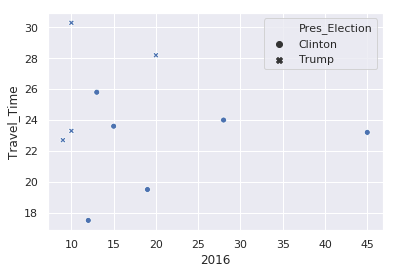
For the first simple example, let’s look at the relationship between the 2016 fatalities and the average Travel_Time . In addition, let’s identify the data based on the Pres_Election column.

sns.scatterplot(x='2016',y='Travel_Time',style='Pres_Election',data=df)
MN Traffic Scatter plot

There are a couple things to note from this example:

  • By using a pandas dataframe, we can just pass in the column names to define the X and Y variables.
  • We can use the same column name approach to alter the marker style .
  • Seaborn takes care of picking a marker style and adding a legend.
  • This approach supports easily changing the views in order to explore the data.

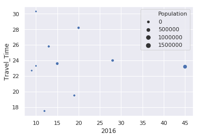
If we’d like to look at the variation by county population:

sns.scatterplot(x='2016',y='Travel_Time',size='Population',data=df)
MN Traffic Scatter plot

In this case, Seaborn buckets the population into 4 categories and adjusts the size of the circle based on that county’s population. A little later in the article, I will show how to adjust the size of the circles so they are larger.

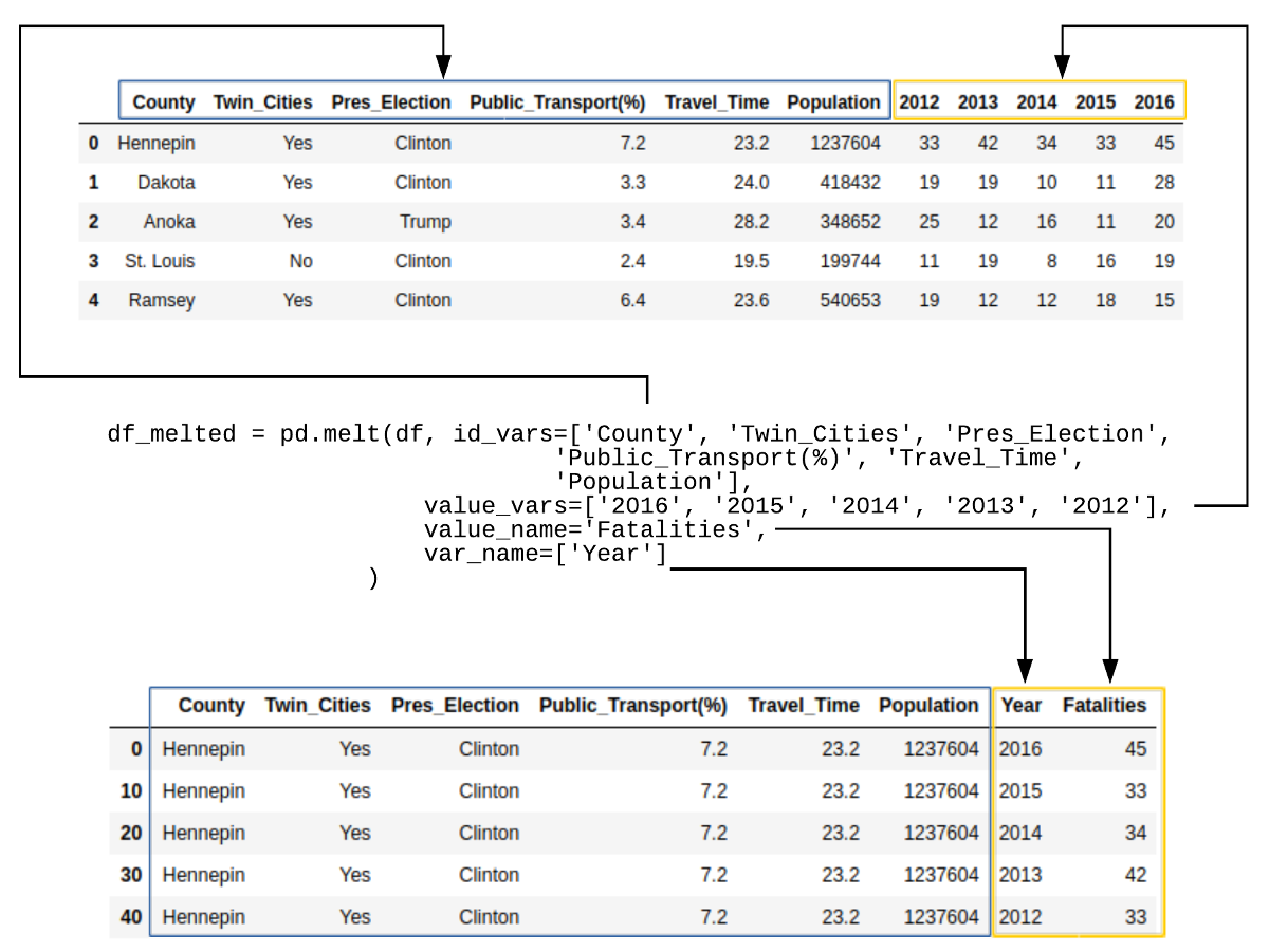
Before we go any further, we need to create a new data frame that contains the data in tidy format. In the original data frame, there is a column for each year that contains the relevant traffic fatality value. Seaborn works much better if the data is structured with the Year and Fatalities in tidy format.

Panda’s handy melt function makes this transformation easy:

df_melted=pd.melt(df,id_vars=['County','Twin_Cities','Pres_Election','Public_Transport(%)','Travel_Time','Population'],value_vars=['2016','2015','2014','2013','2012'],value_name='Fatalities',var_name=['Year'])

Here’s what the data looks like for Hennepin County:

CountyTwin_CitiesPres_ElectionPublic_Transport(%)Travel_TimePopulationYearFatalities
0HennepinYesClinton7.223.21237604201645
10HennepinYesClinton7.223.21237604201533
20HennepinYesClinton7.223.21237604201434
30HennepinYesClinton7.223.21237604201342
40HennepinYesClinton7.223.21237604201233

If this is a little confusing, here is an illustration of what happened:

Melt Example

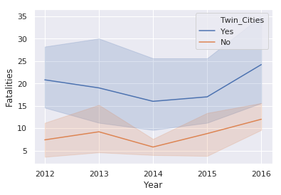
Now that we have the data in tidy format, we can see what the trend of fatalities looks like over time using the new lineplot() function:

sns.lineplot(x='Year',y='Fatalities',data=df_melted,hue='Twin_Cities')
MN Traffic Line Plot

This illustration introduces the hue keyword which changes the color of the line based on the value in the Twin_Cities column. This plot also shows the statistical background inherent in Seaborn plots. The shaded areas are confidence intervals which basically show the range in which our true value lies. Due to the small number of samples, this interval is large.

relplot

A relplot uses the base scatterplot and lineplot to build a FacetGrid. The key feature of a FacetGrid is that it supports creating multiple plots with data varying by rows and columns.

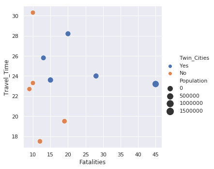
Here’s an example of a scatter plot for the 2016 data:

sns.relplot(x='Fatalities',y='Travel_Time',size='Population',hue='Twin_Cities',sizes=(100,200),data=df_melted.query("Year == '2016'"))
MN Traffic Scatter Plot

This example is similar to the standard scatter plot but there is the added benefit of the legend being placed outside the plot which makes it easier to read. Additionally, I use sizes=(100,200) to scale the circles to a larger value which make them easier to view. Because the data is in tidy format, all years are included. I use the df_melted.query("Year == '2016'") code to filter only on the 2016 data.

The default style for a relplot() is a scatter plot. You can use the kind='line' to use a line plot instead.

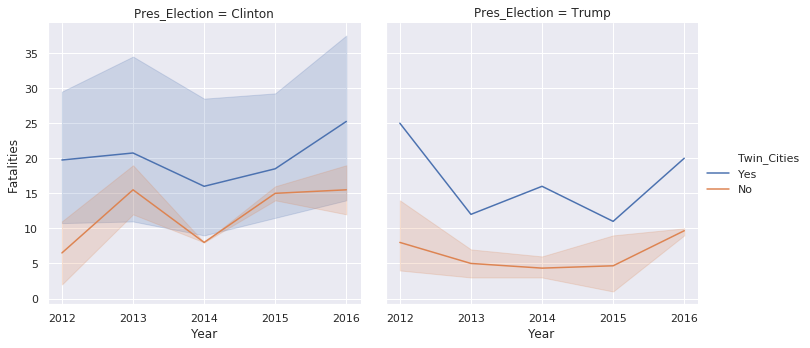
sns.relplot(x='Year',y='Fatalities',data=df_melted,kind='line',hue='Twin_Cities',col='Pres_Election')
MN Traffic Line Plot

This example also shows how the plots can be divided across columns using the col keyword.

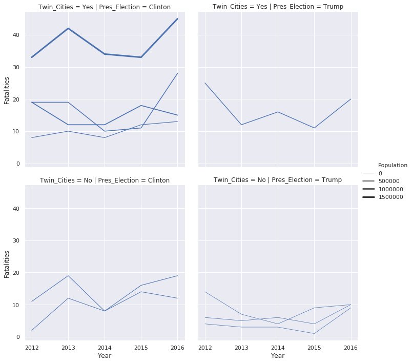
The final example shows how to combine rows, columns, and line size:

sns.relplot(x='Year',y='Fatalities',data=df_melted,kind='line',size='Population',row='Twin_Cities',col='Pres_Election')
MN Traffic Line Plot

Once you get the data into a pandas data frame in tidy format, then you have many different options for plotting your data. Seaborn makes it very easy to look at relationships in many different ways and determine what makes the most sense for your data.

Name Changes

There are only two hard problems in Computer Science: cache invalidation and naming things. — Phil Karlton

In addition to the new features described above, there are some name changes to some of the functions. The biggest change is that factorplot() is now called catplot() and the default catplot() produces a stripplot() as the default plot type. The other big change is that the lvplot() is renamed to a boxenplot(). You can read more about this plot type in the documentation.

Both of these changes might seem minor but names do matter. I think the term “letter-value” plot was not very widely known. Additionally, in python, category plot is a bit more intuitive than the R-terminology based factor plot.

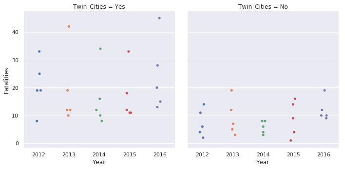
Here’s an example of a default catplot() :

sns.catplot(x='Year',y='Fatalities',data=df_melted,col='Twin_Cities')
MN Traffic Category Plot

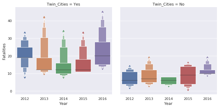
Here’s the same plot using the new boxen plot:

sns.catplot(x='Year',y='Fatalities',data=df_melted,col='Twin_Cities',kind='boxen')
MN Traffic Category Plot

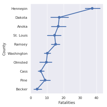
If you would like to replicate the prior default behavior, here’s how to plot a pointplot

sns.catplot(x='Fatalities',y='County',data=df_melted,kind='point')
MN Traffic Point Plot

The categorical plots in seaborn are really useful. They tend to be some of my most frequently used plot types and I am always appreciative of how easy it is to quickly develop different visualizations of the data with minor code changes.

Easter Egg

The author has also included a new plot type called a dogplot() . I’ll shamelessly post the output here in order to gain some sweet sweet traffic to the page:

sns.dogplot()
Dogplot

I don’t know this guy but he definitely looks like a Good Boy!

Final Thoughts

There are several additional features and improvements in this latest release of seaborn. I encourage everyone to review the notes here.

Despite all the changes to existing ones and development of new libraries in the python visualization landscape, seaborn continues to be an extremely important tool for creating beautiful statistical visualizations in python. The latest updates only improve the value of an already useful library.

Python Bytes: #89 A tenacious episode that won't give up

Real Python: Dictionaries in Python

$
0
0

Python provides another composite data type called a dictionary, which is similar to a list in that it is a collection of objects.

Here’s what you’ll learn in this tutorial: You’ll cover the basic characteristics of Python dictionaries and learn how to access and manage dictionary data. Once you have finished this tutorial, you should have a good sense of when a dictionary is the appropriate data type to use, and how to do so.

Dictionaries and lists share the following characteristics:

  • Both are mutable.
  • Both are dynamic. They can grow and shrink as needed.
  • Both can be nested. A list can contain another list. A dictionary can contain another dictionary. A dictionary can also contain a list, and vice versa.

Dictionaries differ from lists in two important ways. The first is the ordering of the elements:

  • Elements in a list have a distinct order, which is an intrinsic property of that list.
  • Dictionaries are unordered. Elements are not kept in any specific order.

The second difference lies in how elements are accessed:

  • List elements are accessed by their position in the list, via indexing.
  • Dictionary elements are accessed via keys.

Defining a Dictionary

Dictionaries are Python’s implementation of a data structure that is more generally known as an associative array. A dictionary consists of a collection of key-value pairs. Each key-value pair maps the key to its associated value.

You can define a dictionary by enclosing a comma-separated list of key-value pairs in curly braces ({}). A colon (:) separates each key from its associated value:

d={<key>:<value>,<key>:<value>,...<key>:<value>}

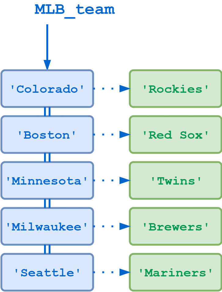
The following defines a dictionary that maps a location to the name of its corresponding Major League Baseball team:

>>> MLB_team={... 'Colorado':'Rockies',... 'Boston':'Red Sox',... 'Minnesota':'Twins',... 'Milwaukee':'Brewers',... 'Seattle':'Mariners'... }
Python dictionary (illustration)Dictionary Mapping Location to MLB Team

You can also construct a dictionary with the built-in dict() function. The argument to dict() should be a sequence of key-value pairs. A list of tuples works well for this:

d=dict([(<key>,<value>),(<key>,<value),...(<key>,<value>)])

MLB_team can then also be defined this way:

>>> MLB_team=dict([... ('Colorado','Rockies'),... ('Boston','Red Sox'),... ('Minnesota','Twins'),... ('Milwaukee','Brewers'),... ('Seattle','Mariners')... ])

If the key values are simple strings, they can be specified as keyword arguments. So here is yet another way to define MLB_team:

>>> MLB_team=dict(... Colorado='Rockies',... Boston='Red Sox',... Minnesota='Twins',... Milwaukee='Brewers',... Seattle='Mariners'... )

Once you’ve defined a dictionary, you can display its contents, the same as you can do for a list. All three of the definitions shown above appear as follows when displayed:

>>> type(MLB_team)<class 'dict'>>>> MLB_team{'Colorado': 'Rockies', 'Boston': 'Red Sox', 'Milwaukee': 'Brewers','Seattle': 'Mariners', 'Minnesota': 'Twins'}

It may seem as though the order in which the key-value pairs are displayed has significance, but remember that dictionaries are unordered collections. They have to print out in some order, of course, but it is effectively random. In the example above, it’s not even the same order in which they were defined.

As you add or delete entries, you won’t be guaranteed that any sort of order will be maintained. But that doesn’t matter, because you don’t access dictionary entries by numerical index:

>>> MLB_team[1]Traceback (most recent call last):
  File "<pyshell#13>", line 1, in <module>MLB_team[1]KeyError: 1

Accessing Dictionary Values

Of course, dictionary elements must be accessible somehow. If you don’t get them by index, then how do you get them?

A value is retrieved from a dictionary by specifying its corresponding key in square brackets ([]):

>>> MLB_team['Minnesota']'Twins'>>> MLB_team['Colorado']'Rockies'

If you refer to a key that is not in the dictionary, Python raises an exception:

>>> MLB_team['Toronto']Traceback (most recent call last):
  File "<pyshell#19>", line 1, in <module>MLB_team['Toronto']KeyError: 'Toronto'

Adding an entry to an existing dictionary is simply a matter of assigning a new key and value:

>>> MLB_team['Kansas City']='Royals'>>> MLB_team{'Colorado': 'Rockies', 'Boston': 'Red Sox', 'Milwaukee': 'Brewers','Seattle': 'Mariners', 'Minnesota': 'Twins', 'Kansas City': 'Royals'}

If you want to update an entry, you can just assign a new value to an existing key:

>>> MLB_team['Seattle']='Seahawks'>>> MLB_team{'Colorado': 'Rockies', 'Boston': 'Red Sox', 'Milwaukee': 'Brewers','Seattle': 'Seahawks', 'Minnesota': 'Twins', 'Kansas City': 'Royals'}

To delete an entry, use the del statement, specifying the key to delete:

>>> delMLB_team['Seattle']>>> MLB_team{'Colorado': 'Rockies', 'Boston': 'Red Sox', 'Milwaukee': 'Brewers','Minnesota': 'Twins', 'Kansas City': 'Royals'}

Begone, Seahawks! Thou art an NFL team.

Dictionary Keys vs. List Indices

You may have noticed that the interpreter raises the same exception, KeyError, when a dictionary is accessed with either an undefined key or by a numeric index:

>>> MLB_team['Toronto']Traceback (most recent call last):
  File "<pyshell#8>", line 1, in <module>MLB_team['Toronto']KeyError: 'Toronto'>>> MLB_team[1]Traceback (most recent call last):
  File "<pyshell#9>", line 1, in <module>MLB_team[1]KeyError: 1

In fact, it’s the same error. In the latter case, [1] looks like a numerical index, but it isn’t.

You will see later in this tutorial that an object of any immutable type can be used as a dictionary key. Accordingly, there is no reason you can’t use integers:

>>> d={0:'a',1:'b',2:'c',3:'d'}>>> d[0]'a'>>> d[2]'c'

In the expressions MLB_team[1], d[0], and d[2], the numbers in square brackets appear as though they might be indices. But Python is interpreting them as dictionary keys. You can’t be guaranteed that Python will maintain dictionary objects in any particular order, and you can’t access them by numerical index. The syntax may look similar, but you can’t treat a dictionary like a list:

>>> type(d)<class 'dict'>>>> d[-1]Traceback (most recent call last):
  File "<pyshell#30>", line 1, in <module>d[-1]KeyError: -1>>> d[0:2]Traceback (most recent call last):
  File "<pyshell#31>", line 1, in <module>d[0:2]TypeError: unhashable type: 'slice'>>> d.append('e')Traceback (most recent call last):
  File "<pyshell#32>", line 1, in <module>d.append('e')AttributeError: 'dict' object has no attribute 'append'

Building a Dictionary Incrementally

Defining a dictionary using curly braces and a list of key-value pairs, as shown above, is fine if you know all the keys and values in advance. But what if you want to build a dictionary on the fly?

You can start by creating an empty dictionary, which is specified by empty curly braces. Then you can add new keys and values one at a time:

>>> person={}>>> type(person)<class 'dict'>>>> person['fname']='Joe'>>> person['lname']='Fonebone'>>> person['age']=51>>> person['spouse']='Edna'>>> person['children']=['Ralph','Betty','Joey']>>> person['pets']={'dog':'Fido','cat':'Sox'}

Once the dictionary is created in this way, its values are accessed the same way as any other dictionary:

>>> person{'fname': 'Joe', 'lname': 'Fonebone', 'age': 51, 'spouse': 'Edna','children': ['Ralph', 'Betty', 'Joey'], 'pets': {'dog': 'Fido', 'cat': 'Sox'}}>>> person['fname']'Joe'>>> person['age']51>>> person['children']['Ralph', 'Betty', 'Joey']

Retrieving the values in the sublist or subdictionary requires an additional index or key:

>>> person['children'][-1]'Joey'>>> person['pets']['cat']'Sox'

This example exhibits another feature of dictionaries: the values contained in the dictionary don’t need to be the same type. In person, some of the values are strings, one is an integer, one is a list, and one is another dictionary.

Just as the values in a dictionary don’t need to be of the same type, the keys don’t either:

>>> foo={42:'aaa',2.78:'bbb',True:'ccc'}>>> foo{42: 'aaa', 2.78: 'bbb', True: 'ccc'}>>> foo[42]'aaa'>>> foo[2.78]'bbb'>>> foo[True]'ccc'

Here, one of the keys is an integer, one is a float, and one is a Boolean. It’s not obvious how this would be useful, but you never know.

Notice how versatile Python dictionaries are. In MLB_team, the same piece of information (the baseball team name) is kept for each of several different geographical locations. person, on the other hand, stores varying types of data for a single person.

You can use dictionaries for a wide range of purposes because there are so few limitations on the keys and values that are allowed. But there are some. Read on!

Restrictions on Dictionary Keys

Almost any type of value can be used as a dictionary key in Python. You just saw this example, where integer, float, and Boolean objects are used as keys:

>>> foo={42:'aaa',2.78:'bbb',True:'ccc'}>>> foo{42: 'aaa', 2.78: 'bbb', True: 'ccc'}

You can even use built-in objects like types and functions:

>>> d={int:1,float:2,bool:3}>>> d{<class 'int'>: 1, <class 'float'>: 2, <class 'bool'>: 3}>>> d[float]2>>> d={bin:1,hex:2,oct:3}>>> d[oct]3

However, there are a couple restrictions that dictionary keys must abide by.

First, a given key can appear in a dictionary only once. Duplicate keys are not allowed. A dictionary maps each key to a corresponding value, so it doesn’t make sense to map a particular key more than once.

You saw above that when you assign a value to an already existing dictionary key, it does not add the key a second time, but replaces the existing value:

>>> MLB_team={... 'Colorado':'Rockies',... 'Boston':'Red Sox',... 'Minnesota':'Twins',... 'Milwaukee':'Brewers',... 'Seattle':'Mariners'... }>>> MLB_team['Minnesota']='Timberwolves'>>> MLB_team{'Colorado': 'Rockies', 'Boston': 'Red Sox', 'Minnesota': 'Timberwolves','Milwaukee': 'Brewers', 'Seattle': 'Mariners'}

Similarly, if you specify a key a second time during the initial creation of a dictionary, the second occurrence will override the first:

>>> MLB_team={... 'Colorado':'Rockies',... 'Boston':'Red Sox',... 'Minnesota':'Timberwolves',... 'Milwaukee':'Brewers',... 'Seattle':'Mariners',... 'Minnesota':'Twins'... }>>> MLB_team{'Colorado': 'Rockies', 'Boston': 'Red Sox', 'Minnesota': 'Twins','Milwaukee': 'Brewers', 'Seattle': 'Mariners'}

Begone, Timberwolves! Thou art an NBA team. Sort of.

Secondly, a dictionary key must be of a type that is immutable. That means an integer, float, string, or Boolean can be a dictionary key, as you have seen above. A tuple can also be a dictionary key, because tuples are immutable:

>>> d={(1,1):'a',(1,2):'b',(2,1):'c',(2,2):'d'}>>> d[(1,1)]'a'>>> d[(2,1)]'c'

Recall from the discussion on tuples that one rationale for using a tuple instead of a list is that there are circumstances where an immutable type is required. This is one of them.

However, neither a list nor another dictionary can serve as a dictionary key, because lists and dictionaries are mutable:

>>> d={[1,1]:'a',[1,2]:'b',[2,1]:'c',[2,2]:'d'}Traceback (most recent call last):
  File "<pyshell#20>", line 1, in <module>d={[1,1]:'a',[1,2]:'b',[2,1]:'c',[2,2]:'d'}TypeError: unhashable type: 'list'

Technical Note: Why does the error message say “unhashable” rather than “mutable”? Python uses hash values internally to implement dictionary keys, so an object must be hashable to be used as a key.

See the Python Glossary for more information.

Restrictions on Dictionary Values

By contrast, there are no restrictions on dictionary values. Literally none at all. A dictionary value can be any type of object Python supports, including mutable types like lists and dictionaries, and user-defined objects, which you will learn about in upcoming tutorials.

There is also no restriction against a particular value appearing in a dictionary multiple times:

>>> d={0:'a',1:'a',2:'a',3:'a'}>>> d{0: 'a', 1: 'a', 2: 'a', 3: 'a'}>>> d[0]==d[1]==d[2]True

Operators and Built-in Functions

You have already become familiar with many of the operators and built-in functions that can be used with strings, lists, and tuples. Some of these work with dictionaries as well.

For example, the in and not in operators return True or False according to whether the specified operand occurs as a key in the dictionary:

>>> MLB_team={... 'Colorado':'Rockies',... 'Boston':'Red Sox',... 'Minnesota':'Twins',... 'Milwaukee':'Brewers',... 'Seattle':'Mariners'... }>>> 'Milwaukee'inMLB_teamTrue>>> 'Toronto'inMLB_teamFalse>>> 'Toronto'notinMLB_teamTrue

You can use the in operator together with short-circuit evaluation to avoid raising an error when trying to access a key that is not in the dictionary:

>>> MLB_team['Toronto']Traceback (most recent call last):
  File "<pyshell#2>", line 1, in <module>MLB_team['Toronto']KeyError: 'Toronto'>>> 'Toronto'inMLB_teamandMLB_team['Toronto']False

In the second case, due to short-circuit evaluation, the expression MLB_team['Toronto'] is not evaluated, so the KeyError exception does not occur.

The len() function returns the number of key-value pairs in a dictionary:

>>> MLB_team={... 'Colorado':'Rockies',... 'Boston':'Red Sox',... 'Minnesota':'Twins',... 'Milwaukee':'Brewers',... 'Seattle':'Mariners'... }>>> len(MLB_team)5

Built-in Dictionary Methods

As with strings and lists, there are several built-in methods that can be invoked on dictionaries. In fact, in some cases, the list and dictionary methods share the same name. (In the discussion on object-oriented programming, you will see that it is perfectly acceptable for different types to have methods with the same name.)

The following is an overview of methods that apply to dictionaries:

d.clear()

Clears a dictionary.

d.clear() empties dictionary d of all key-value pairs:

>>> d={'a':10,'b':20,'c':30}>>> d{'a': 10, 'b': 20, 'c': 30}>>> d.clear()>>> d{}

d.get(<key>[, <default>])

Returns the value for a key if it exists in the dictionary.

The .get() method provides a convenient way of getting the value of a key from a dictionary without checking ahead of time whether the key exists, and without raising an error.

d.get(<key>) searches dictionary d for <key> and returns the associated value if it is found. If <key> is not found, it returns None:

>>> d={'a':10,'b':20,'c':30}>>> print(d.get('b'))20>>> print(d.get('z'))None

If <key> is not found and the optional <default> argument is specified, that value is returned instead of None:

>>> print(d.get('z',-1))-1

d.items()

Returns a list of key-value pairs in a dictionary.

d.items() returns a list of tuples containing the key-value pairs in d. The first item in each tuple is the key, and the second item is the key’s value:

>>> d={'a':10,'b':20,'c':30}>>> d{'a': 10, 'b': 20, 'c': 30}>>> list(d.items())[('a', 10), ('b', 20), ('c', 30)]>>> list(d.items())[1][0]'b'>>> list(d.items())[1][1]20

d.keys()

Returns a list of keys in a dictionary.

d.keys() returns a list of all keys in d:

>>> d={'a':10,'b':20,'c':30}>>> d{'a': 10, 'b': 20, 'c': 30}>>> list(d.keys())['a', 'b', 'c']

d.values()

Returns a list of values in a dictionary.

d.values() returns a list of all values in d:

>>> d={'a':10,'b':20,'c':30}>>> d{'a': 10, 'b': 20, 'c': 30}>>> list(d.values())[10, 20, 30]

Any duplicate values in d will be returned as many times as they occur:

>>> d={'a':10,'b':10,'c':10}>>> d{'a': 10, 'b': 10, 'c': 10}>>> list(d.values())[10, 10, 10]

Technical Note: The .items(), .keys(), and .values() methods actually return something called a view object. A dictionary view object is more or less like a window on the keys and values. For practical purposes, you can think of these methods as returning lists of the dictionary’s keys and values.

d.pop(<key>[, <default>])

Removes a key from a dictionary, if it is present, and returns its value.

If <key> is present in d, d.pop(<key>) removes <key> and returns its associated value:

>>> d={'a':10,'b':20,'c':30}>>> d.pop('b')20>>> d{'a': 10, 'c': 30}

d.pop(<key>) raises a KeyError exception if <key> is not in d:

>>> d={'a':10,'b':20,'c':30}>>> d.pop('z')Traceback (most recent call last):
  File "<pyshell#4>", line 1, in <module>d.pop('z')KeyError: 'z'

If <key> is not in d, and the optional <default> argument is specified, then that value is returned, and no exception is raised:

>>> d={'a':10,'b':20,'c':30}>>> d.pop('z',-1)-1>>> d{'a': 10, 'b': 20, 'c': 30}

d.popitem()

Removes a key-value pair from a dictionary.

d.popitem() removes a random, arbitrary key-value pair from d and returns it as a tuple:

>>> d={'a':10,'b':20,'c':30}>>> d.popitem()('c', 30)>>> d{'a': 10, 'b': 20}>>> d.popitem()('b', 20)>>> d{'a': 10}

If d is empty, d.popitem() raises a KeyError exception:

>>> d={}>>> d.popitem()Traceback (most recent call last):
  File "<pyshell#11>", line 1, in <module>d.popitem()KeyError: 'popitem(): dictionary is empty'

d.update(<obj>)

Merges a dictionary with another dictionary or with an iterable of key-value pairs.

If <obj> is a dictionary, d.update(<obj>) merges the entries from <obj> into d. For each key in <obj>:

  • If the key is not present in d, the key-value pair from <obj> is added to d.
  • If the key is already present in d, the corresponding value in d for that key is updated to the value from <obj>.

Here is an example showing two dictionaries merged together:

>>> d1={'a':10,'b':20,'c':30}>>> d2={'b':200,'d':400}>>> d1.update(d2)>>> d1{'a': 10, 'b': 200, 'c': 30, 'd': 400}

In this example, key 'b' already exists in d1, so its value is updated to 200, the value for that key from d2. However, there is no key 'd' in d1, so that key-value pair is added from d2.

<obj> may also be a sequence of key-value pairs, similar to when the dict() function is used to define a dictionary. For example, <obj> can be specified as a list of tuples:

>>> d1={'a':10,'b':20,'c':30}>>> d1.update([('b',200),('d',400)])>>> d1{'a': 10, 'b': 200, 'c': 30, 'd': 400}

Or the values to merge can be specified as a list of keyword arguments:

>>> d1={'a':10,'b':20,'c':30}>>> d1.update(b=200,d=400)>>> d1{'a': 10, 'b': 200, 'c': 30, 'd': 400}

Conclusion

In this tutorial, you covered the basic properties of the Python dictionary and learned how to access and manipulate dictionary data.

Lists and dictionaries are two of the most frequently used Python types. As you have seen, they differ from one another in the following ways:

TypeElement OrderElement Access
ListOrderedBy index
DictionaryUnorderedBy key

Because of their differences, lists and dictionaries tend to be appropriate for different circumstances. You should now have a good feel for which, if either, would be best for a given situation.

Next you will learn about Python sets. The set is another unordered composite data type, but it is quite different from a dictionary.


[ Improve Your Python With 🐍 Python Tricks 💌 – Get a short & sweet Python Trick delivered to your inbox every couple of days. >> Click here to learn more and see examples ]


Curtis Miller: Learn Foundations of Python Natural Language Processing and Computer Vision with my Video Course: Applications of Statistical Learning with Python

$
0
0
This final course caps the series off with applications. The first half of the course covers two major areas of AI: natural language processing (NLP) and computer vision (CV). In the NLP section, I introduce basic NLP tasks and show how to use Python's Natural Language Toolkit (NLTK) for NLP. Then in the CV section I show several CV tasks and how to use libraries from PIL to OpenCV and SciPy. These sections are brief in theory and heavy in application; nearly every video includes an extensive Python application of the concepts and software presented. The last two sections of the course are complete Python projects. The first project is an NLP project; the objective is to train a spam detector. The second project develops a system for detecting emotions in images. In these projects, I get a dataset, prepare it for processing, apply a machine learning system and evaluate the results. These projects use techniques and concepts from all the previous courses in the series (though one may be able to appreciate the content without having seen the other courses).

NumFOCUS: Optimization modeling language JuMP joins NumFOCUS Sponsored Projects

Codementor: Looking for Python mentor / guidance

$
0
0
Hi everyone! I am fairly new to the coding side of this work - I've worked the last year or two on cyber and tech policy at the governmental level, but am switching towards work in a NGO...

Kushal Das: vcrpy for web related tests

$
0
0

Couple of weeks ago, Jen pointed me to vcrpy. This is a Python implementation of Ruby’s library with same name.

What is vcrpy?

It is a Python module which helps to write faster and simple tests involving HTTP requests. It records all the HTTP interactions in plain text files (by default in a YAML file). This helps to write deterministic tests, and also to run them in offline.

It works well with the following Python modules.

  • requests
  • aiohttp
  • urllib3
  • tornado
  • urllib2
  • boto3

Usage example

Let us take a very simple test case.

import unittest
import requests

class TestExample(unittest.TestCase):

    def test_httpget(self):
        r = requests.get("https://httpbin.org/get?name=vcrpy&lang=Python")
        self.assertEqual(r.status_code, 200)
        data = r.json()
        self.assertEqual(data["args"]["name"], "vcrpy")
        self.assertEqual(data["args"]["lang"], "Python")


if __name__ == "__main__":
    unittest.main()

In the above code, we are making a HTTP GET request to the https://httpbin.org site and examining the returned JSON data. Running the test takes around 1.75 seconds in my computer.

$ python test_all.py
.
------------------------------------------------------------------
Ran 1 test in 1.752s

OK

Now, we can add vcrpy to this project.

import unittest
import vcr
import requests

class TestExample(unittest.TestCase):

    @vcr.use_cassette("test-httpget.yml")
    def test_httpget(self):
        r = requests.get("https://httpbin.org/get?name=vcrpy&lang=Python")
        self.assertEqual(r.status_code, 200)
        data = r.json()
        self.assertEqual(data["args"]["name"], "vcrpy")
        self.assertEqual(data["args"]["lang"], "Python")

if __name__ == "__main__":
    unittest.main()

We imported vcr module, and added a decorator vcr.use_cassette to our test function. Now, when we will execute the test again, vcrpy will record the HTTP call details in the mentioned YAML file, and use the same for the future test runs.

$ python test_all.py
.
------------------------------------------------------------------
Ran 1 test in 0.016s

OK

You all can also notice the time taken to run the test, around 0.2 second.

Read the project documentation for all the available options.

Codementor: Python Tuples and Tuple Methods

$
0
0
Lists and tuples are standard Python data types that store values in a sequence. Atuple is immutable whereas a list is mutable. Here are some other advantages of tuples over lists (partially from Stack Overflow (https://stackoverflow.com/questions/1708510/python-list-vs-tuple-when-to-use-each))

Codementor: Setup Microservices Architecture in Python with ZeroMQ & Docker

$
0
0
Microservices - What? Microservices (https://en.wikipedia.org/wiki/Microservices) are an architectural style in which multiple, independent processes communicate with each other. These processes...

Matthew Rocklin: Building SAGA optimization for Dask arrays

$
0
0

This work is supported by ETH Zurich, Anaconda Inc, and the Berkeley Institute for Data Science

At a recent Scikit-learn/Scikit-image/Dask sprint at BIDS, Fabian Pedregosa (a machine learning researcher and Scikit-learn developer) and Matthew Rocklin (Dask core developer) sat down together to develop an implementation of the incremental optimization algorithm SAGA on parallel Dask datasets. The result is a sequential algorithm that can be run on any dask array, and so allows the data to be stored on disk or even distributed among different machines.

It was interesting both to see how the algorithm performed and also to see the ease and challenges to run a research algorithm on a Dask distributed dataset.

Start

We started with an initial implementation that Fabian had written for Numpy arrays using Numba. The following code solves an optimization problem of the form

importnumpyasnpfromnumbaimportnjitfromsklearn.linear_model.sagimportget_auto_step_sizefromsklearn.utils.extmathimportrow_norms@njitdefderiv_logistic(p,y):# derivative of logistic loss# same as in lightning (with minus sign)p*=yifp>0:phi=1./(1+np.exp(-p))else:exp_t=np.exp(p)phi=exp_t/(1.+exp_t)return(phi-1)*y@njitdefSAGA(A,b,step_size,max_iter=100):"""
  SAGA algorithm

  A : n_samples x n_features numpy array
  b : n_samples numpy array with values -1 or 1
  """n_samples,n_features=A.shapememory_gradient=np.zeros(n_samples)gradient_average=np.zeros(n_features)x=np.zeros(n_features)# vector of coefficientsstep_size=0.3*get_auto_step_size(row_norms(A,squared=True).max(),0,'log',False)for_inrange(max_iter):# sample randomlyidx=np.arange(memory_gradient.size)np.random.shuffle(idx)# .. inner iteration ..foriinidx:grad_i=deriv_logistic(np.dot(x,A[i]),b[i])# .. update coefficients ..delta=(grad_i-memory_gradient[i])*A[i]x-=step_size*(delta+gradient_average)# .. update memory terms ..gradient_average+=(grad_i-memory_gradient[i])*A[i]/n_samplesmemory_gradient[i]=grad_i# monitor convergenceprint('gradient norm:',np.linalg.norm(gradient_average))returnx

This implementation is a simplified version of the SAGA implementation that Fabian uses regularly as part of his research, and that assumes that $f$ is the logistic loss, i.e., $f(z) = \log(1 + \exp(-z))$. It can be used to solve problems with other values of $f$ by overwriting the function deriv_logistic.

We wanted to apply it across a parallel Dask array by applying it to each chunk of the Dask array, a smaller Numpy array, one at a time, carrying along a set of parameters along the way.

Development Process

In order to better understand the challenges of writing Dask algorithms, Fabian did most of the actual coding to start. Fabian is good example of a researcher who knows how to program well and how to design ML algorithms, but has no direct exposure to the Dask library. This was an educational opportunity both for Fabian and for Matt. Fabian learned how to use Dask, and Matt learned how to introduce Dask to researchers like Fabian.

Step 1: Build a sequential algorithm with pure functions

To start we actually didn’t use Dask at all, instead, Fabian modified his implementation in a few ways:

  1. It should operate over a list of Numpy arrays. A list of Numpy arrays is similar to a Dask array, but simpler.
  2. It should separate blocks of logic into separate functions, these will eventually become tasks, so they should be sizable chunks of work. In this case, this led to the creating of the function _chunk_saga that performs an iteration of the SAGA algorithm on a subset of the data.
  3. These functions should not modify their inputs, nor should they depend on global state. All information that those functions require (like the parameters that we’re learning in our algorithm) should be explicitly provided as inputs.

These requested modifications affect performance a bit, we end up making more copies of the parameters and more copies of intermediate state. In terms of programming difficulty this took a bit of time (around a couple hours) but is a straightforward task that Fabian didn’t seem to find challenging or foreign.

These changes resulted in the following code:

fromnumbaimportnjitfromsklearn.utils.extmathimportrow_normsfromsklearn.linear_model.sagimportget_auto_step_size@njitdef_chunk_saga(A,b,n_samples,f_deriv,x,memory_gradient,gradient_average,step_size):# Make explicit copies of inputsx=x.copy()gradient_average=gradient_average.copy()memory_gradient=memory_gradient.copy()# Sample randomlyidx=np.arange(memory_gradient.size)np.random.shuffle(idx)# .. inner iteration ..foriinidx:grad_i=f_deriv(np.dot(x,A[i]),b[i])# .. update coefficients ..delta=(grad_i-memory_gradient[i])*A[i]x-=step_size*(delta+gradient_average)# .. update memory terms ..gradient_average+=(grad_i-memory_gradient[i])*A[i]/n_samplesmemory_gradient[i]=grad_ireturnx,memory_gradient,gradient_averagedeffull_saga(data,max_iter=100,callback=None):"""
  data: list of (A, b), where A is a n_samples x n_features
  numpy array and b is a n_samples numpy array
  """n_samples=0forA,bindata:n_samples+=A.shape[0]n_features=data[0][0].shape[1]memory_gradients=[np.zeros(A.shape[0])for(A,b)indata]gradient_average=np.zeros(n_features)x=np.zeros(n_features)steps=[get_auto_step_size(row_norms(A,squared=True).max(),0,'log',False)for(A,b)indata]step_size=0.3*np.min(steps)for_inrange(max_iter):fori,(A,b)inenumerate(data):x,memory_gradients[i],gradient_average=_chunk_saga(A,b,n_samples,deriv_logistic,x,memory_gradients[i],gradient_average,step_size)ifcallbackisnotNone:print(callback(x,data))returnx

Step 2: Apply dask.delayed

Once functions neither modified their inputs nor relied on global state we went over a dask.delayed example, and then applied the @dask.delayed decorator to the functions that Fabian had written. Fabian did this at first in about five minutes and to our mutual surprise, things actually worked

@dask.delayed(nout=3)# <<<---- New@njitdef_chunk_saga(A,b,n_samples,f_deriv,x,memory_gradient,gradient_average,step_size):...deffull_saga(data,max_iter=100,callback=None):n_samples=0forA,bindata:n_samples+=A.shape[0]data=dask.persist(*data)# <<<---- New...for_inrange(max_iter):fori,(A,b)inenumerate(data):x,memory_gradients[i],gradient_average=_chunk_saga(A,b,n_samples,deriv_logistic,x,memory_gradients[i],gradient_average,step_size)cb=dask.delayed(callback)(x,data)# <<<---- Changedx,cb=dask.persist(x,cb)# <<<---- Newprint(cb.compute()

However, they didn’t work that well. When we took a look at the dask dashboard we find that there is a lot of dead space, a sign that we’re still doing a lot of computation on the client side.

Step 3: Diagnose and add more dask.delayed calls

While things worked, they were also fairly slow. If you notice the dashboard plot above you’ll see that there is plenty of white in between colored rectangles. This shows that there are long periods where none of the workers is doing any work.

This is a common sign that we’re mixing work between the workers (which shows up on the dashbaord) and the client. The solution to this is usually more targetted use of dask.delayed. Dask delayed is trivial to start using, but does require some experience to use well. It’s important to keep track of which operations and variables are delayed and which aren’t. There is some cost to mixing between them.

At this point Matt stepped in and added delayed in a few more places and the dashboard plot started looking cleaner.

@dask.delayed(nout=3)# <<<---- New@njitdef_chunk_saga(A,b,n_samples,f_deriv,x,memory_gradient,gradient_average,step_size):...deffull_saga(data,max_iter=100,callback=None):n_samples=0forA,bindata:n_samples+=A.shape[0]n_features=data[0][0].shape[1]data=dask.persist(*data)# <<<---- Newmemory_gradients=[dask.delayed(np.zeros)(A.shape[0])for(A,b)indata]# <<<---- Changedgradient_average=dask.delayed(np.zeros)(n_features)#  Changedx=dask.delayed(np.zeros)(n_features)# <<<---- Changedsteps=[dask.delayed(get_auto_step_size)(dask.delayed(row_norms)(A,squared=True).max(),0,'log',False)for(A,b)indata]# <<<---- Changedstep_size=0.3*dask.delayed(np.min)(steps)# <<<---- Changedfor_inrange(max_iter):fori,(A,b)inenumerate(data):x,memory_gradients[i],gradient_average=_chunk_saga(A,b,n_samples,deriv_logistic,x,memory_gradients[i],gradient_average,step_size)cb=dask.delayed(callback)(x,data)# <<<---- Changedx,memory_gradients,gradient_average,step_size,cb= \
            dask.persist(x,memory_gradients,gradient_average,step_size,cb)# Newprint(cb.compute())# <<<---- changedreturnx

From a dask perspective this now looks good. We see that one partial_fit call is active at any given time with no large horizontal gaps between partial_fit calls. We’re not getting any parallelism (this is just a sequential algorithm) but we don’t have much dead space. The model seems to jump between the various workers, processing on a chunk of data before moving on to new data.

Step 4: Profile

The dashboard image above gives confidence that our algorithm is operating as it should. The block-sequential nature of the algorithm comes out cleanly, and the gaps between tasks are very short.

However, when we look at the profile plot of the computation across all of our cores (Dask constantly runs a profiler on all threads on all workers to get this information) we see that most of our time is spent compiling Numba code.

We started a conversation for this on the numba issue tracker which has since been resolved. That same computation over the same time now looks like this:

The tasks, which used to take seconds, now take tens of milliseconds, so we can process through many more chunks in the same amount of time.

Future Work

This was a useful experience to build an interesting algorithm. Most of the work above took place in an afternoon. We came away from this activity with a few tasks of our own:

  1. Build a normal Scikit-Learn style estimator class for this algorithm so that people can use it without thinking too much about delayed objects, and can instead just use dask arrays or dataframes
  2. Integrate some of Fabian’s research on this algorithm that improves performance with sparse data and in multi-threaded environments.
  3. Think about how to improve the learning experience so that dask.delayed can teach new users how to use it correctly

Talk Python to Me: #173 Coming into Python from another Industry (part 1)

$
0
0
Not everyone comes to software development and Python through 4-year computer science programs at universities. This episode highlights one alternative journey into Python.

Python Bytes: #90 A Django Async Roadmap

Nikola: Nikola v8.0.0b3 is out!

$
0
0

On behalf of the Nikola team, I am pleased to announce the immediate availability of Nikola v8.0.0b3. This is the third and hopefully final beta of Nikola v8. The big change in this release is the adoption of Babel to handle date translations (instead of relying on system locale, which didn’t work well for us). Other issues and bugs were fixed.

Many themes in our Index have been ported for Nikola v8, but some of them are not yet there.

What is Nikola?

Nikola is a static site and blog generator, written in Python. It can use Mako and Jinja2 templates, and input in many popular markup formats, such as reStructuredText and Markdown — and can even turn Jupyter Notebooks into blog posts! It also supports image galleries, and is multilingual. Nikola is flexible, and page builds are extremely fast, courtesy of doit (which is rebuilding only what has been changed).

Find out more at the website: https://getnikola.com/

Downloads

Install using pip install Nikola==8.0.0b3.

If you want to upgrade to Nikola v8, make sure to read the Upgrading blog post.

Changes

Features

  • New data_file option for chart shortcode and directive (Issue #3129)
  • Show the filename of the missing file when nikola serve can't find a file (i.e. when an 404 error occurs).
  • Better error messages for JSON download failures in nikola plugin and nikola theme (Issue getnikola/plugins#282)
  • Use Babel instead of the locale module to better handle localizations (Issues #2606, #3121)
  • Change DATE_FORMAT formats to CLDR formats (Issue #2606)

Bugfixes

  • Fix listing installed themes if theme directory is missing.
  • Watch correct output folder in nikola auto (Issue #3119)
  • Fix post fragment dependencies when posts are only available in a non-default language (Issue #3112)
  • Implement MARKDOWN_EXTENSION_CONFIGS properly (Issue #2970)
  • Ignore .DS_Store when processing listings (Issue #3099)
  • Remove redundant check for tag similarity (Mentioned in Issue #3123)

Bhishan Bhandari: Python map() built-in

$
0
0

Map makes an iterator that takes a function and uses the arguments from the following iterables passed to the map built-in. What makes this possible is the equal status of every object in Python. One of the main goals of Python was to have an equal status for all the objects. Remember how even a […]

The post Python map() built-in appeared first on The Tara Nights.

Mike Driscoll: Python 101: Episode #19 – The subprocess module

Viewing all 22647 articles
Browse latest View live


<script src="https://jsc.adskeeper.com/r/s/rssing.com.1596347.js" async> </script>