In this post, we will go through Decision Tree model building. We will use air quality data. Here is the link to data.
importpandasaspdimportnumpyasnp# Reading our csv datacombine_data=pd.read_csv('data/Real_combine.csv')combine_data.head(5)T == Average Temperature (°C)
TM == Maximum temperature (°C)
Tm == Minimum temperature (°C)
SLP == Atmospheric pressure at sea level (hPa)
H == Average relative humidity (%)
VV == Average visibility (Km)
V == Average wind speed (Km/h)
VM == Maximum sustained wind speed (Km/h)
PM2.5== Fine particulate matter (PM2.5) is an air pollutant that is a concern for people's health when levels in air are high
Let us drop first the unwanted columns.
combine_data.drop(['Unnamed: 0'],axis=1,inplace=True)combine_data.head(2)# combine data top 5 rowscombine_data.head()# combine data bottom 5 featurescombine_data.tail()Let us print the statistical data using describe() function.
# To get statistical data combine_data.describe()Let us check if there are any null values in our data.
combine_data.isnull().sum()we can also visualize null values with seaborn too. From the heatmap, it is clear that there are no null values.
importseabornassnssns.heatmap(combine_data.isnull(),yticklabels=False)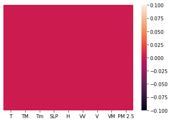
Let us check outliers in our data using seaborn boxplot.
# To check outliers importmatplotlib.pyplotasplta4_dims=(11.7,8.27)fig,ax=plt.subplots(figsize=a4_dims)g=sns.boxplot(data=combine_data,linewidth=2.5,ax=ax)g.set_yscale("log")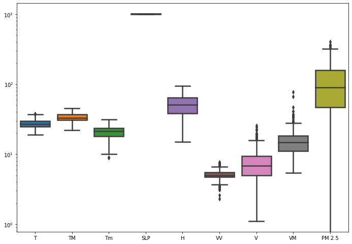
From the plot, we can see that there are few outliers present in column Tm, W, V, VM and PM 2.5.
We can also do a searborn pairplot multivariate analysis. Using multivariate analysis, we can find out relation between any two variables. Since plot is so big, i am skipping the pairplot, but the command to draw pairplots are shown below.
sns.pairplot(combine_data)We can also check the corelation between dependent and independent features using dataframe.corr() function. The correlation can be plotted using 'pearson', 'kendall, or 'spearman'. By default corr() function runs 'pearson'.
combine_data.corr()If we observe the above correlation table, it is clear that correlation between 'PM 2.5' feature and only SLP is positive. Corelation tells us if 'PM 2.5' increases what is the behaviour of other features. So if correlation is negative that means if one variable increases other variable decreases.
We can also Visualize Correlation Using Seaborn Heatmap.
relation=combine_data.corr()relation_index=relation.indexrelation_indexsns.heatmap(combine_data[relation_index].corr(),annot=True)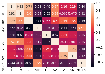
Upto now, we have done only feature engineering. In next section, we will do feature selection.
fromsklearn.ensembleimportRandomForestRegressorfromsklearn.model_selectionimporttrain_test_splitfromsklearn.metricsimportmean_squared_errorasmseSplitting the data into train and test data sets.
X_train,X_test,y_train,y_test=train_test_split(combine_data.iloc[:,:-1],combine_data.iloc[:,-1],test_size=0.3,random_state=0)# size of train data setX_train.shape# size of test data setX_test.shapeFeature selection by ExtraTreesRegressor(model based). ExtraTreesRegressor helps us find the features which are most important.
# Feature selection by ExtraTreesRegressor(model based)fromsklearn.ensembleimportExtraTreesRegressorfromsklearn.model_selectionimporttrain_test_splitfromsklearn.metricsimportaccuracy_scoreasaccX_train,X_test,y_train,y_test=train_test_split(combine_data.iloc[:,:-1],combine_data.iloc[:,-1],test_size=0.3,random_state=0)reg=ExtraTreesRegressor()reg.fit(X_train,y_train)Letusprintthefeaturesimportance.reg.feature_importances_feat_importances=pd.Series(reg.feature_importances_,index=X_train.columns)feat_importances.nlargest(5).plot(kind='barh')plt.show()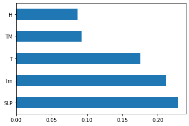
Based on plot above, we can select the features which will be most important for our prediction model.
Before Train the data we need to do feature normalization because models such as decision trees are very sensitive to the scale of features.
# Traning model with all features fromsklearn.model_selectionimporttrain_test_splitX_train,X_test,y_train,y_test=train_test_split(combine_data.iloc[:,:-1],combine_data.iloc[:,-1],test_size=0.3,random_state=0)X_trainX_testfromsklearn.treeimportDecisionTreeRegressorLet us creat a Decision tree regression model.
reg_decision_model=DecisionTreeRegressor()# fit independent varaibles to the dependent variablesreg_decision_model.fit(X_train,y_train)reg_decision_model.score(X_train,y_train)reg_decision_model.score(X_test,y_test)We got 100% score on training data.
On test data we got 5.7% score because we did not provide any tuning parameters while intializing the tree as a result of which algorithm split the training data till the leaf node. Due to which depth of tree increased and our model did the overfitting.
That's why we are getting high score on our training data and less score on test data.
So to solve this problem we would use hyper parameter tuning.
We can use GridSearch or RandomizedSearch for hyper parameters tuning.
prediction=reg_decision_model.predict(X_test)Let us do a distribution plot between our label y and predicted y values.
# checking difference between labled y and predicted ysns.distplot(y_test-prediction)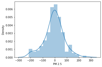
We are getting nearly bell shape curve that means our model working good? No we can't make that conclusion. Good bell curve only tell us the range of predicted values are with in the same range as our original data range values are.
checkingpredictedyandlabeledyusingascatterplot.plt.scatter(y_test,prediction)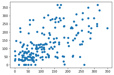
# Hyper parameters range intialization for tuning parameters={"splitter":["best","random"],"max_depth":[1,3,5,7,9,11,12],"min_samples_leaf":[1,2,3,4,5,6,7,8,9,10],"min_weight_fraction_leaf":[0.1,0.2,0.3,0.4,0.5,0.6,0.7,0.8,0.9],"max_features":["auto","log2","sqrt",None],"max_leaf_nodes":[None,10,20,30,40,50,60,70,80,90]}Above we intialized hyperparmeters random range using Gridsearch to find the best parameters for our decision tree model.
# calculating different regression metricsfromsklearn.model_selectionimportGridSearchCVtuning_model=GridSearchCV(reg_decision_model,param_grid=parameters,scoring='neg_mean_squared_error',cv=3,verbose=3)# function for calculating how much time take for hyperparameter tuningdeftimer(start_time=None):ifnotstart_time:start_time=datetime.now()returnstart_timeelifstart_time:thour,temp_sec=divmod((datetime.now()-start_time).total_seconds(),3600)tmin,tsec=divmod(temp_sec,60)#print(thour,":",tmin,':',round(tsec,2))X=combine_data.iloc[:,:-1]y=combine_data.iloc[:,-1]%%capture
from datetime import datetime
start_time=timer(None)
tuning_model.fit(X,y)
timer(start_time)
Hyper parameter tuning took around 17 minues. It might vary depending upon your machine.
# best hyperparameters tuning_model.best_params_# best model scoretuning_model.best_score_tuned_hyper_model=DecisionTreeRegressor(max_depth=5,max_features='auto',max_leaf_nodes=50,min_samples_leaf=2,min_weight_fraction_leaf=0.1,splitter='random')# fitting modeltuned_hyper_model.fit(X_train,y_train)# prediction tuned_pred=tuned_hyper_model.predict(X_test)plt.scatter(y_test,tuned_pred)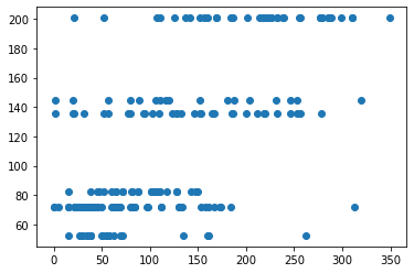
Ok the above scatter plot looks lot better.
Let us compare now Error rate of our model with hyper tuning of paramerters to our original model which is without the tuning of parameters.
# With hyperparameter tuned fromsklearnimportmetricsprint('MAE:',metrics.mean_absolute_error(y_test,tuned_pred))print('MSE:',metrics.mean_squared_error(y_test,tuned_pred))print('RMSE:',np.sqrt(metrics.mean_squared_error(y_test,tuned_pred)))# without hyperparameter tuning fromsklearnimportmetricsprint('MAE:',metrics.mean_absolute_error(y_test,prediction))print('MSE:',metrics.mean_squared_error(y_test,prediction))print('RMSE:',np.sqrt(metrics.mean_squared_error(y_test,prediction)))If you observe the above metrics for both the models, We got good metric values(MSE 4155) with hyperparameter tuning model compare to model without hyper parameter tuning.