This is a simple example for custom print output.
The script detect the platform for color settings and then use print.
The first print will print with blue color the name of the script.
I used random to select a random color from colors array and used to print the -=RANDOM COLOR=- text.
The print (W+'') is used to set default white color for terminal
import sys
import random
if sys.platform == "
↧
Catalin George Festila: Python 3.7.4 : Print with random colors.
↧
Python Software Foundation: PyPI Security Q4 2019 Request for Proposals period opens.
The Python Software Foundation Packaging Working Group has received a grant from Facebook Research to implement advanced security features for PyPI. These features include cryptographic signing of uploaded artifacts and the infrastructure necessary to implement automated detection of malicious files uploaded to the index.
![]()
![]()
![]()
![]()
![]()
The Python Package Index (PyPI) is a foundational component of the Python ecosystem and broader computer software and technology landscape. This project aims to improve the security and accessibility of PyPI for all users worldwide, whether they are direct users, like project maintainers and
pip installers, or indirect users. The impact of this work will be highly visible and improve crucial features of the service.
We plan to begin the project in Quarter 4 of 2019. Because of the size of the project, funding has been allocated to secure one or more contractors to complete the development, testing, verification, and assist in the rollout of necessary features.
Timeline
| Date | Milestone |
|---|---|
| September 25 | Request for Proposal period opened. |
| October 21 | Request for Proposal period closes. |
| October 29 | Date proposals will have received a decision. |
| December 2 | Contract work commences. |
What is the Request for Proposals period?
A Request for Proposal (RFP) is a process intended to allow us (The Python Software Foundation) to collect proposals from potential contractors and select contractor(s) best suited to fulfill the specified work.
After the RFP period closes we will evaluate the received proposals based on the evaluation criteria, seek clarification from proposers as necessary, and select one or more contractors to complete the work specified in the scope.
The Request for Proposals period opens today, September 25th, 2019, and is scheduled to close October 21, 2019 AoE.
How do I submit a proposal?
First, please read the full contents of the Request for Proposals here!
You'll find the instructions for submission, evaluation criteria, as well as scope of the project there.
↧
↧
Robin Wilson: Automatically annotating a boxplot in matplotlib
You can probably tell from the sudden influx of matplotlib posts that I've been doing a lot of work plotting graphs recently...
I have produced a number of boxplots to compare different sets of data. Some of these graphs are for a non-technical audience, and my client agreed that a boxplot was the best way to visualise the data, but wanted the various elements of the boxplot to be labelled so the audience could work out how to interpret it.
I started doing this manually using the plt.annotate function, but quickly got fed up with manually positioning everything - so I wrote a quick function to do it for me.
If you just want the code then here it is - it's not perfect, but it should be a good starting point for you:
def annotate_boxplot(bpdict, annotate_params=None,
x_offset=0.05, x_loc=0,
text_offset_x=35,
text_offset_y=20):
"""Annotates a matplotlib boxplot with labels marking various centile levels.
Parameters:
- bpdict: The dict returned from the matplotlib `boxplot` function. If you're using pandas you can
get this dict by setting `return_type='dict'` when calling `df.boxplot()`.
- annotate_params: Extra parameters for the plt.annotate function. The default setting uses standard arrows
and offsets the text based on other parameters passed to the function
- x_offset: The offset from the centre of the boxplot to place the heads of the arrows, in x axis
units (normally just 0-n for n boxplots). Values between around -0.15 and 0.15 seem to work well
- x_loc: The x axis location of the boxplot to annotate. Usually just the number of the boxplot, counting
from the left and starting at zero.
text_offset_x: The x offset from the arrow head location to place the associated text, in 'figure points' units
text_offset_y: The y offset from the arrow head location to place the associated text, in 'figure points' units
"""
if annotate_params is None:
annotate_params = dict(xytext=(text_offset_x, text_offset_y), textcoords='offset points', arrowprops={'arrowstyle':'->'})
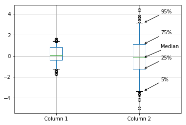
plt.annotate('Median', (x_loc + 1 + x_offset, bpdict['medians'][x_loc].get_ydata()[0]), **annotate_params)
plt.annotate('25%', (x_loc + 1 + x_offset, bpdict['boxes'][x_loc].get_ydata()[0]), **annotate_params)
plt.annotate('75%', (x_loc + 1 + x_offset, bpdict['boxes'][x_loc].get_ydata()[2]), **annotate_params)
plt.annotate('5%', (x_loc + 1 + x_offset, bpdict['caps'][x_loc*2].get_ydata()[0]), **annotate_params)
plt.annotate('95%', (x_loc + 1 + x_offset, bpdict['caps'][(x_loc*2)+1].get_ydata()[0]), **annotate_params)You can then run code like this:
df = pd.DataFrame({'Column 1': np.random.normal(size=100),
                   'Column 2': np.random.normal(scale=2, size=100)})

bpdict = df.boxplot(whis=[5, 95], return_type='dict')
annotate_boxplot(bpdict, x_loc=1)
This will produce something like this:
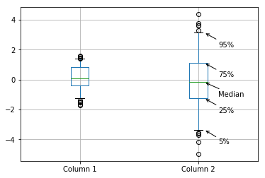
You can pass various parameters to change the display. For example, to make the labels closer to the boxplot and lower than the thing they're pointing at, set the parameters as: text_offset_x=20 and text_offset_y=-20, giving:
So, how does this work? Well, when you create a boxplot, matplotlib very helpfully returns you a dict containing the matplotlib objects referring to each part of the boxplot: the box, the median line, the whiskers etc. It looks a bit like this:
{'boxes': [<matplotlib.lines.Line2D object at 0x1179db908>,
           <matplotlib.lines.Line2D object at 0x1176ac3c8>],
 'caps': [<matplotlib.lines.Line2D object at 0x117736668>,
          <matplotlib.lines.Line2D object at 0x1177369b0>,
          <matplotlib.lines.Line2D object at 0x1176acda0>,
          <matplotlib.lines.Line2D object at 0x1176ace80>],
 'fliers': [<matplotlib.lines.Line2D object at 0x117736dd8>,
            <matplotlib.lines.Line2D object at 0x1176b07b8>],
 'means': [],
 'medians': [<matplotlib.lines.Line2D object at 0x117736cf8>,
             <matplotlib.lines.Line2D object at 0x1176b0470>],
 'whiskers': [<matplotlib.lines.Line2D object at 0x11774ef98>,
              <matplotlib.lines.Line2D object at 0x117736320>,
              <matplotlib.lines.Line2D object at 0x1176ac710>,
              <matplotlib.lines.Line2D object at 0x1176aca58>]}
Each of these objects is a matplotlib.lines.Line2D object, which has a get_xdata() and get_ydata() method (see the docs for more details). In this case, all we're interested in is the y locations, so get_ydata() suffices.
All we do then is grab the right co-ordinate from the list of co-ordinates that are returned (noting that for the box we have to look at the 0th and the 2nd co-ordinates to get the bottom and top of the box respectively). We also have to remember that the caps dict entry has two objects for each individual boxplot - as there are caps at the bottom and the top - so we have to be a bit careful with selecting those.
The other useful thing to point out is that you can choose what co-ordinate systems you use with the plt.annotate function - so you can set textcoords='offset points' and then set the same xytext value each time we call it - and all the labels will be offset from their arrowhead location the same amount. That saves us manually calculating a location for the text each time.
This function was gradually expanded to allow more configurability - and could be expanded a lot more, but should work as a good starting point for anyone wanting to do the same sort of thing. It depends on a lot of features of plt.annotate - for more details on how to use this function look at its documentation or the Advanced Annotation guide.
↧
Codementor: How I built a Python script to read e-mails from an Exchange Server
Python script to read e-mail in Exchange
↧
Python Software Foundation: Felipe de Morais: 2019 Q2 Community Service Award Winner
Pythonistas everywhere benefit when our community reflects the many backgrounds and experiences of Python’s users. However it can be challenging to participate in the community when there are no local user groups or harder yet if groups do exist but you do not feel represented in them. After learning that a friend was experiencing gender descrimination at work, Felipe de Morais of Porto Alegre, Brazil, decided to start Django Girls Porto Alegre. By starting this group, women like his friend who were facing similar challenges could have a community to call their own.
Since Django Girls Porto Alegre took off in 2015, it has become one of the most active Django Girls groups in the world. Inspired by Django Girls and PyLadies, Felipe also started AfroPython, an initiative to empower Black people through technology. Additionally, Felipe contributes to Operação Serenata de Amor, an open source project that monitors public spending by politicians. For this work the PSF is pleased to award Felipe de Morais with the Q2 2019 Community Service Award:
Felipe grew up in Rio De Janeiro where he earned a graduate degree in Computer Science and later moved to Porto Alegre in southern Brazil. With a strong desire to be part of a community, Felipe traveled to IT-related Meetup groups but longed for more accessible means to network and teach. Python was his go-to language for its simplicity and ease, and he loved to teach the language to help other people along in their careers. It is no surprise that the groups he’s started have both a Python and inclusivity focus.
When asked about his motivation for starting Python groups, Felipe says that that he simply gets great joy out of helping people. “I've seen people starting their work life because the workshop unlocked this career path for them,'' he says. “The most important part of it is the relationships made along the way, which make a great support system for a lot of people making positive life changes.”
Renata D'Avila, a Django Girls Porto Alegre organizer, met Felipe 2016 at a Hackerspace event and the two have kept in touch ever since. “He is one of the people behind one of the biggest Django Girls workshop ever organized.” she recalls, “Django Girls Porto Alegre 2017 had about 180 people involved, among participants, mentors, and organizers.” However the event, as most events do, encountered some bumps in the road. As lunchtime rolled around and the planned caterers never showed up, Felipe raced across campus and resolved the issue, returning to the event with enough food for everyone. “That was one of the greatest achievements of that huge workshop,” says Renata, “that everyone could eat and that the schedule for the workshop was kept without people even knowing about how much effort it took to make it work.”
Since Django Girls Porto Alegre took off in 2015, it has become one of the most active Django Girls groups in the world. Inspired by Django Girls and PyLadies, Felipe also started AfroPython, an initiative to empower Black people through technology. Additionally, Felipe contributes to Operação Serenata de Amor, an open source project that monitors public spending by politicians. For this work the PSF is pleased to award Felipe de Morais with the Q2 2019 Community Service Award:
RESOLVED, that the Python Software Foundation award the Q2 2019 Community Service Award to Felipe de Morais for his work towards facilitating the growth of the Python Brazilian community by organizing workshops, contributing to open source code that benefits the Brazilian people and for setting an example for all community organizers.
Felipe grew up in Rio De Janeiro where he earned a graduate degree in Computer Science and later moved to Porto Alegre in southern Brazil. With a strong desire to be part of a community, Felipe traveled to IT-related Meetup groups but longed for more accessible means to network and teach. Python was his go-to language for its simplicity and ease, and he loved to teach the language to help other people along in their careers. It is no surprise that the groups he’s started have both a Python and inclusivity focus.
When asked about his motivation for starting Python groups, Felipe says that that he simply gets great joy out of helping people. “I've seen people starting their work life because the workshop unlocked this career path for them,'' he says. “The most important part of it is the relationships made along the way, which make a great support system for a lot of people making positive life changes.”
 |
| AfroPython 2017 |
 |
| AfroPython 2018 |
In May of 2017 when Felipe was attending Python Sudeste, a regional Python event in southeastern Brazil, he met Jessica Temporal. Jessica had been working as a data scientist on a large political open-source project, Operação Serenata de Amor. Serenata analyzes open data from the Brazilian government and flags expenses made by elected politicians that might be unlawful. Jessica was organizing a sprint at the conference and Felipe jumped in to help. In addition to working on some important refactoring and code readability issues, “Felipe was significant in making the project more friendly to newcomers,'' she says. He continues to contribute to the project today.
 |
| Felipe (left) with Seranata founder Eduardo Cuducos (middle) and Seranata data scientist Jessica Temporal (right) |
 |
| CSA Award Winner Felipe de Morais |
↧
↧
Codementor: ML with Python: Part-2
In this Post, we will cover in detail what we do in various steps involved in creating a machine learning (ML) model. I was looking around some ML project which is not very complex but covers all...
↧
PyCharm: 2019.3 EAP 3
A new version of the Early Access Program (EAP) for PyCharm 2019.3 is available now! Download it from our website.
New for this version
Literal types support
Python 3.8 release is right around the corner and we are working on supporting its latest features. PyCharm 2019.3 EAP 3 introduces the support for Literal types. Literal types is Python 3.8’s new alternative to define type signatures for functions (PEP-0586). With this now you have the ability to indicate that some expression expects a specific and concrete value.

Further improvements
- Our stub support was extended to support proper code autocompletion for modules like ‘sys’, ‘logging’, ‘concurrent’ and ’email’.
- An issue causing the output of a Jupyter notebook not to render properly was fixed.
- We renamed the tabs for the Jupyter toolwindow to avoid confusions. Now it will more obvious that the outer one refers to the process and the inner one to its output.
- For more details on what’s new in this version, see the release notes
Interested?
Download this EAP from our website. Alternatively, you can use the JetBrains Toolbox App to stay up to date throughout the entire EAP.
If you’re on Ubuntu 16.04 or later, you can use snap to get PyCharm EAP, and stay up to date. You can find the installation instructions on our website.
↧
PyCharm: Webinar Recording: “10 Tools and Techniques Python Web Developers Should Explore” with Michael Kennedy
Our friend Michael Kennedy joined us yesterday for a webinar on tips every Python web developer could benefit from. As is usual with his webinars, it was a lot of fun, very well-prepared, and packed a ton of useful information. The recording is now available as well as his repository of examples.
During the webinar, Michael covered the following material:
- 1:50: HTML5 Form Features
- 7:40: ngrok
- 14:57: async/await
- 28:49: Database Migrations
- 42:27: Vue.js for rich frontend
- 46:52: View Models
- 50:32: Docker
- 53:24: letsencrypt for SSL
- 59:33: secure.py
- 1:00:20: Wrapup
Further material is available: previous webinar on async/await, his course on concurrency, his course on MongoDB, his “Effective PyCharm” book with Matt Harrison, and his Mastering PyCharm course, in addition to his podcasts.
Thanks again Michael for helping PyCharm users get up-to-speed on these important topics.
↧
Dataquest: Write Better Code With Our New Advanced Functions Python Course
Learning to write better code — code that's readable, maintainable, and debuggable — is a crucial skill for being an effective part of a data science team.
The post Write Better Code With Our New Advanced Functions Python Course appeared first on Dataquest.
↧
↧
Red Hat Developers: Python wheels, AI/ML, and ABI compatibility
Python has become a popular programming language in the AI/ML world. Projects like TensorFlow and PyTorch have Python bindings as the primary interface used by data scientists to write machine learning code. However, distributing AI/ML-related Python packages and ensuring application binary interface (ABI) compatibility between various Python packages and system libraries presents a unique set of challenges.
The manylinux standard (e.g., manylinux2014) for Python wheels provides a practical solution to these challenges, but it also introduces new challenges that the Python community and developers need to consider. Before we delve into these additional challenges, we’ll briefly look at the Python ecosystem for packaging and distribution.
Wheels, AI/ML, and ABIs
Python packages are installed using the pip command, which downloads the package from pypi.org.
pip install <package-name>
These packages can be of two types:
- Pure Python wheels, which may or may not be targeted to a specific Python version
- Extension wheels, which use native code written in C/C++
All AI/ML Python packages are extension wheels that use native operating system libraries. Compiled Python extension modules built on one distribution may not work on other distributions, or even on different machines running the same distribution with different system libraries installed. This is because the compiled binaries have a record of the ABI they rely on, such as relocations, symbols and versions, size of global data symbols, etc. At runtime, if the ABI does not match, the loader may raise an error. An example of a missing symbol with a version would look like this:
/lib64/libfoo.so.1: version `FOO_1.2' not found (required by ./app)
AI/ML project maintainers need to build different Python packages for Windows, macOS X, and Linux distributions. The precompiled binaries are packaged in a wheel format with the .whl file extension. A wheel is a zip file that can be interpreted as a Python library.
The file name contains specific tags, which are used by the pip command to determine the Python version and operating system that match the system on which the AI/ML library is installed. The wheel also contains the layout of a Python project as it should be installed on the system. To avoid the need for users to compile these packages the project maintainers build and upload platform-specific wheels for Windows, macOS, and Linux on pypi.org.
Here are some examples of wheels for Linux and non-Linux distros:
tensorflow-2.0.0-cp27-cp27m-macosx_10_11_x86_64.whl
tensorflow-2.0.0-cp35-cp35m-win_amd64.whl
tensorflow-2.0.0-cp36-cp36m-manylinux1_x86_64.whl
tensorflow-2.0.0-cp37-cp37m-manylinux2010_x86_64.whl
Manylinux2014
AI/ML project maintainers who want to distribute the Python library with native code for Linux distros have the difficult task of ensuring ABI compatibility. The compiled code needs to run on a wide variety of Linux distributions.
Fortunately, there is a way to make a binary compatible with most (though not all) Linux distributions. To do this, you need to build a binary and use an ABI baseline that is older than any distribution you want to support. The expectation is that the newer distributions will keep the ABI guarantees; that way, you’ll be able to run your binary on newer distributions as long as they provide the ABI baseline. Eventually, the ABI baselines will change in an incompatible way, and that may be a technical requirement for moving the baseline forward. There are other non-technical requirements for moving the ABI baseline forward, and they revolve around distribution lifecycles.
The manylinux platform tag is a way to make your Python libraries that are compatible with most Linux distributions. Python’s manylinux defines an ABI baseline and targets the baseline by building on an old version of a distribution. To achieve maximum compatibility, it uses the longest-supported freely distributable version of Linux: CentOS.
The first manylinux platform tag called manylinux1 uses CentOS 5. The second iteration called manylinux2010 uses CentOS 6. The latest specification manylinux2014 is a result of Red Hat, other vendors, and the Python community moving the manylinux specification ahead to use CentOS 7/UBI 7 and support more architectures.
To make the life of AI/ML Python project maintainers easier, the Python community provides a prebuilt manylinux build container, which can be used to build project wheels, listed here:
centos5 Image - quay.io/pypa/manylinux1_x86_64
centos6 Image - quay.io/pypa/manylinux2010_x86_64
ubi7 Image - quay.io/pypa/manylinux2014_x86_64(coming soon)
For AI/ML Python project users the pip command is very important. The pip command will install the appropriate wheel file based on wheel tags and also based on the manylinux platform tag of the wheel which matches the system. For example, a manylinux2014 wheel will not install on Red Hat Enterprise Linux (RHEL) 6 because it doesn’t have the system library versions specified in the manylinux2014 specification. Pip will install manylinux2010 wheels on RHEL 6 and manylinux2014 wheels on RHEL 7.
AI/ML Python project users have to ensure they update pip command regularly before they update to the next AI/ML Python project version. If users are using containers, then the latest pip command should be available in the container.
Additional challenges
Although the manylinux standard has helped deliver reliable and stable extension wheels, it does introduce two additional challenges:
- Lifecycle
At some point, the reference platforms for the ABI baselines will have end-of-life. The Python community must actively track the end-of-life support and CVEs for different system libraries used by the project and potentially move project maintainers to the next available manylinux platform tag. Note: The EOL for CentOS 6 is November 30, 2020. The EOL for CentOS 7 is June 30, 2024.
Lastly, project maintainers should ensure that they build wheels for all the manylinux platform tags or at least the wheels of the most recent specifications. This will give users the most options for installation. - Hardware vendor support
Almost all AI/ML Python projects have some form of hardware accelerator support, such as CUDA (NVIDIA), ROCm (AMD), Intel MKL. The hardware vendors might not support all versions of the toolchain and project maintainers should pick a baseline toolchain (gcc, binutils, glibc) and set their wheels to a certain manylinux platform tags that match. Some projects might need to support a variety of architectures including Intel/AMD (i686, x86_64), Arm (aarch64, armhfp), IBM POWER (ppc64, ppc64le), or IBM Z Series (s390x). Regression tests on different architectures are essential to catch compatibility issues. See the Red Hat Enterprise Linux ABI compatibility guides for RHEL 7 and RHEL 8.
Solutions
The Python community must follow the lifecycle of the reference software that is used to target the ABI baselines and plan accordingly. Python developers must carefully match system tooling or developer tooling to the hardware vendor software requirements. Solving both of these is a difficult but ultimately rewarding challenge.

The post Python wheels, AI/ML, and ABI compatibility appeared first on Red Hat Developer.
↧
Yasoob Khalid: Looking for an internship for Summer 2020
Hi lovely people!  Hope everything is going well on your end. I asked you guys last year for helping me find a kick-ass internship and you all came through. I ended up working at ASAPP over the summer and had an awesome time. I wrote an article about what I learned during my internship.
I am putting out the same request for next summer as well. If you have benefited from any of my articles and work at an amazing company and feel like I would be a good addition to your team, please reach out. I am looking for a 12-14 week internship from around mid-May to mid-August in 2020. I strongly prefer small teams where I can bond with the people I am working with. I am open to most places but bonus points if you work at a hardware based tech company or a fintech startup. However, this is not a hard requirement.
If you are working at an innovative company in some major European country and can sponsor Visa, I would be really interested in that as well!
I have done a lot of backend development in Python and GoLang. I am fairly comfortable with dabbling in the front-end code as well. I have also tinkered with open source hardware (Arduino & Raspberry Pi) and wrote a coupleofarticles about what I did and how I did it. You can take a look at my resume (PDF) to get a better understanding of my expertise. You can also read about how I got into programming through this article.
tldr: I love working with exciting stuff even if it means I have to learn something completely new!
I hope you guys would come through this time as well. Have a fantastic day and keep smiling. If you have any questions/comments/suggestions, please comment below or send me an email at yasoob.khld at gmail.com.
See ya! 
↧
Nathan Piccini Data Science Dojo Blog: 101 Data Science Interview Questions, Answers, and Key Concepts

In October 2012, the Harvard Business Review described “Data Scientist” as the “sexiest” job of the 21st century. Well, as we approach 2020 the description still holds true! The world needs more data scientists than there are available for hire. All companies - from the smallest to the biggest - want to hire for a job role that has something “Data” in its name: “Data Scientists”, “Data Analysts”, “Data Engineers” etc.
On the other hand, there's large number of people who are trying to get a break in the Data Science industry, including people with considerable experience in other functional domains such as marketing, finance, insurance, and software engineering. You might have already invested in learning data science (maybe even at a data science bootcamp), but how confident are you for your next Data Science interview?
This blog is intended to give you a nice tour of the questions asked in a Data Science interview. After thorough research, we have compiled a list of 101 actual data science interview questions that have been asked between 2016-2019 at some of the largest recruiters in the data science industry – Amazon, Microsoft, Facebook, Google, Netflix, Expedia, etc.
If you want to know more regarding the tips and tricks for acing the interviews, watch the data science interview AMA with some of our own Data Scientists.
Data Science is an interdisciplinary field and sits at the intersection of computer science, statistics/mathematics, and domain knowledge. To be able to perform well, one needs to have a good foundation in not one but multiple fields, and it reflects in the interview. We've divided the questions into 6 categories:
- Machine Learning
- Data Analysis
- Statistics, Probability, and Mathematics
- Programming
- SQL
- Experiential/Behavioral Questions
We've also provided brief answers and key concepts for each question. Once you've gone through all the questions, you'll have a good understanding of how well you're prepared for your next data science interview!
Machine Learning
As one will expect, data science interviews focus heavily on questions that help the company test your concepts, applications, and experience on machine learning. Each question included in this category has been recently asked in one or more actual data science interviews at companies such as Amazon, Google, Microsoft, etc. These questions will give you a good sense of what sub-topics appear more often than others. You should also pay close attention to the way these questions are phrased in an interview.
Data Analysis
Machine learning concepts are not the only area in which you'll be tested in the interview. Data pre-processing and data exploration are other areas where you can always expect a few questions. We're grouping all such questions under this category. Data analysis is the process of evaluating data using analytical and statistical tools to discover useful insights. Once again, all these questions have been recently asked in one or more actual data science interviews at the companies listed above.
Statistics, Probability and Mathematics
As we've already mentioned, data science builds its foundation on statistics and probability concepts. Having a strong foundation in statistics and probability concepts is a requirement for data science, and these topics are always brought up in data science interviews. Here is a list of statistics and probability questions that have been asked in actual data science interviews.
Programming
When you appear for a data science interview your interviewers are not expecting you to come up with a highly efficient code that takes the lowest resources on computer hardware and executes it quickly. However, they do expect you to be able to use R, Python, or SQL programming languages so that you can access the data sources and at least build prototypes for solutions.
You should expect a few programming/coding questions in your data science interviews. You interviewer might want you to write a short piece of code on a whiteboard to assess how comfortable you are with coding, as well as get a feel for how many lines of codes you typically write in a given week.
Here are some programming and coding questions that companies like Amazon, Google, and Microsoft have asked in their data science interviews.
Structured Query Language (SQL)
Real-world data is stored in databases and it ‘travels’ via queries. If there's one language a data science professional must know, it's SQL - or “Structured Query Language”. SQL is widely used across all job roles in data science and is often a ‘deal-breaker’. SQL questions are placed early on in the hiring process and used for screening. Here are some SQL questions that top companies have asked in their data science interviews.
Situational/Behavioral Questions
Capabilities don’t necessarily guarantee performance. It's for this reason employers ask you situational or behavioral questions in order to assess how you would perform in a given situation. In some cases, a situational or behavioral question would force you to reflect on how you behaved and performed in a past situation. A situational question can help interviewers in assessing your role in a project you might have included in your resume, can reveal whether or not you're a team player, or how you deal with pressure and failure. Situational questions are no less important than any of the technical questions, and it will always help to do some homework beforehand. Recall your experience and be prepared!
Here are some situational/behavioral questions that large tech companies typically ask:
Thanks for reading! We hope this list is able to help you prepare and eventually ace the interview!
Like the 101 machine learning algorithms blog post, the accordion drop down lists are available for you to embed on your own site/blog post. Simply click the 'embed' button in the lower left-hand corner, copy the iframe, and paste it within the page.
↧
Rickard Lindberg: Segfault with custom events in wxPython
Segfault with custom events in wxPython
Published on 2019-09-28.
When working on porting Timeline to Python 3, I ran into a problem where a test caused a segfault. I managed to create a small example that reproduces the failure. I describe the example below and show how I solved the test failure.
The example consists of a test that stores an instance of a custom wx event in a mock object:
- test_wx.py
fromunittest.mockimportMockimportunittestimportwximportwx.lib.neweventCustomEvent,EVT_CUSTOM=wx.lib.newevent.NewEvent()classWxTest(unittest.TestCase):deftest_wx(self):mock=Mock()mock.PostEvent(CustomEvent())if__name__=="__main__":unittest.main()
When I run this example, I get the following error:
$python3test_wx.py.----------------------------------------------------------------------Ran1testin0.001sOKSegmentationfault(coredumped)
If I instead run it through gdb, I can see the C stacktrace where the error happens:
$gdbpython3GNUgdb(GDB)Fedora8.2.91.20190401-23.fc30...(gdb)runtest_wx.py....----------------------------------------------------------------------Ran1testin0.001sOKProgramreceivedsignalSIGSEGV,Segmentationfault.dict_dealloc(mp=0x7fffe712f9d8)at/usr/src/debug/python3-3.7.3-1.fc30.x86_64/Objects/dictobject.c:19011901/usr/src/debug/python3-3.7.3-1.fc30.x86_64/Objects/dictobject.c:Nosuchfileordirectory.Missingseparatedebuginfos,use:dnfdebuginfo-installfontconfig-2.13.1-6.fc30.x86_64libXcursor-1.1.15-5.fc30.x86_64libgcrypt-1.8.4-3.fc30.x86_64libxkbcommon-0.8.3-1.fc30.x86_64lz4-libs-1.8.3-2.fc30.x86_64python3-sip-4.19.17-1.fc30.x86_64(gdb)bt#0dict_dealloc(mp=0x7fffe712f9d8)at/usr/src/debug/python3-3.7.3-1.fc30.x86_64/Objects/dictobject.c:1901#10x00007fffea02e1ccinwxPyEvtDict::~wxPyEvtDict(this=0x5555556f3ee8,__in_chrg=<optimizedout>)at../../../../src/pyevent.h:48#2wxPyEvent::~wxPyEvent(this=0x5555556f3e90,__in_chrg=<optimizedout>)at../../../../src/pyevent.h:96#3sipwxPyEvent::~sipwxPyEvent(this=0x5555556f3e90,__in_chrg=<optimizedout>)at../../../../sip/cpp/sip_corewxPyEvent.cpp:56#40x00007fffea02e24dinsipwxPyEvent::~sipwxPyEvent(this=0x5555556f3e90,__in_chrg=<optimizedout>)at../../../../sip/cpp/sip_corewxPyEvent.cpp:56#50x00007fffea02dfd2inrelease_wxPyEvent(sipCppV=0x5555556f3e90,sipState=<optimizedout>)at../../../../sip/cpp/sip_corewxPyEvent.cpp:261#60x00007fffe72ff4cein??()from/usr/lib64/python3.7/site-packages/sip.so#70x00007fffe72ff51din??()from/usr/lib64/python3.7/site-packages/sip.so#80x00007ffff7c14869insubtype_dealloc(self=<_Eventatremote0x7fffea4ddd38>)at/usr/src/debug/python3-3.7.3-1.fc30.x86_64/Objects/typeobject.c:1256#90x00007ffff7b8892bintupledealloc(op=0x7fffe712cda0)at/usr/src/debug/python3-3.7.3-1.fc30.x86_64/Objects/tupleobject.c:246#100x00007ffff7b8892bintupledealloc(op=0x7fffea4d7620)at/usr/src/debug/python3-3.7.3-1.fc30.x86_64/Objects/tupleobject.c:246#110x00007ffff7c14869insubtype_dealloc(self=<_Callatremote0x7fffea4d7620>)at/usr/src/debug/python3-3.7.3-1.fc30.x86_64/Objects/typeobject.c:1256#120x00007ffff7b882aeinlist_dealloc(op=0x7fffe70ba228)at/usr/src/debug/python3-3.7.3-1.fc30.x86_64/Objects/listobject.c:324#130x00007ffff7c14869insubtype_dealloc(self=<_CallListatremote0x7fffe70ba228>)at/usr/src/debug/python3-3.7.3-1.fc30.x86_64/Objects/typeobject.c:1256#140x00007ffff7b8c813infree_keys_object(keys=0x555555855080)at/usr/src/debug/python3-3.7.3-1.fc30.x86_64/Modules/gcmodule.c:776#15dict_dealloc(mp=0x7fffe712f630)at/usr/src/debug/python3-3.7.3-1.fc30.x86_64/Objects/dictobject.c:1913#16subtype_clear(self=<optimizedout>)at/usr/src/debug/python3-3.7.3-1.fc30.x86_64/Objects/typeobject.c:1101#17delete_garbage(old=<optimizedout>,collectable=<optimizedout>)at/usr/src/debug/python3-3.7.3-1.fc30.x86_64/Modules/gcmodule.c:769#18collect(generation=2,n_collected=0x7fffffffd230,n_uncollectable=0x7fffffffd228,nofail=0)at/usr/src/debug/python3-3.7.3-1.fc30.x86_64/Modules/gcmodule.c:924#190x00007ffff7c4ac4eincollect_with_callback(generation=generation@entry=2)at/usr/src/debug/python3-3.7.3-1.fc30.x86_64/Modules/gcmodule.c:1036#200x00007ffff7ca7331inPyGC_Collect()at/usr/src/debug/python3-3.7.3-1.fc30.x86_64/Modules/gcmodule.c:1581#210x00007ffff7caaf03inPy_FinalizeEx()at/usr/src/debug/python3-3.7.3-1.fc30.x86_64/Python/pylifecycle.c:1185#220x00007ffff7cab048inPy_Exit(sts=sts@entry=0)at/usr/src/debug/python3-3.7.3-1.fc30.x86_64/Python/pylifecycle.c:2278#230x00007ffff7cab0ffinhandle_system_exit()at/usr/src/debug/python3-3.7.3-1.fc30.x86_64/Python/pythonrun.c:636#240x00007ffff7cab1e6inPyErr_PrintEx(set_sys_last_vars=1)at/usr/src/debug/python3-3.7.3-1.fc30.x86_64/Python/pythonrun.c:646#250x00007ffff7cab651inPyRun_SimpleFileExFlags(fp=<optimizedout>,filename=<optimizedout>,closeit=<optimizedout>,flags=0x7fffffffd410)at/usr/src/debug/python3-3.7.3-1.fc30.x86_64/Python/pythonrun.c:435#260x00007ffff7cad864inpymain_run_file(p_cf=0x7fffffffd410,filename=<optimizedout>,fp=0x5555555a20d0)at/usr/src/debug/python3-3.7.3-1.fc30.x86_64/Modules/main.c:427#27pymain_run_filename(cf=0x7fffffffd410,pymain=0x7fffffffd520)at/usr/src/debug/python3-3.7.3-1.fc30.x86_64/Modules/main.c:1627#28pymain_run_python(pymain=0x7fffffffd520)at/usr/src/debug/python3-3.7.3-1.fc30.x86_64/Modules/main.c:2877#29pymain_main(pymain=0x7fffffffd520)at/usr/src/debug/python3-3.7.3-1.fc30.x86_64/Modules/main.c:3038#300x00007ffff7cadc0cin_Py_UnixMain(argc=<optimizedout>,argv=<optimizedout>)at/usr/src/debug/python3-3.7.3-1.fc30.x86_64/Modules/main.c:3073#310x00007ffff7e12f33in__libc_start_main(main=0x555555555050<main>,argc=2,argv=0x7fffffffd678,init=<optimizedout>,fini=<optimizedout>,rtld_fini=<optimizedout>,stack_end=0x7fffffffd668)at../csu/libc-start.c:308#320x000055555555508ein_start()
Somewhere in the middle, there is a call to PyGC_Collect followed, a bit higher up, by a call to release_wxPyEvent. This indicates that the error occurs during garbage collection of the custom wx event.
The machine I run the example on is running Python 3.7.3, and wxPython 4.0.4:
$python3Python3.7.3(default,Mar272019,13:36:35)[GCC9.0.120190227(RedHat9.0.1-0.8)]onlinuxType"help","copyright","credits"or"license"formoreinformation.>>>importwx>>>wx.version()'4.0.4gtk3(phoenix)wxWidgets3.0.4'
To solve this problem, I replaced the mock function PostEvent with one that simply discards its input like this:
mock.PostEvent=lambdax:None
This way there is no custom wx event to garbage collect. In Timeline's case, it was not important to store the event in the mock object anyway.
If you have any idea why this example causes a segfault, I would be interested to know. It feels like an error in the wxPython wrapper.
↧
↧
Test and Code: 89: Improving Programming Education - Nicholas Tollervey
Nicholas Tollervey is working toward better ways of teaching programming. His projects include the Mu Editor, PyperCard, and CodeGrades. Many of us talk about problems with software education. Nicholas is doing something about it.
Special Guest: Nicholas Tollervey.
Sponsored By:
- Azure Pipelines: Automate your builds and deployments with pipelines so you spend less time with the nuts and bolts and more time being creative. Many organizations and open source projects are using Azure Pipelines already. Get started for free at azure.com/pipelines
Support Test & Code - Python Testing & Development
Links:
- Code With Mu— a simple Python editor for beginner programmers
- Made With Mu— A blog to celebrate projects that use the Mu Python code editor to create cool stuff.
- PyperCard— Easy GUIs for All
- CodeGrades
↧
Codementor: Data Cleaning In Python Basics Using Pandas
This post will give you a basic introduction on cleaning data in Python using the pandas library.
↧
Peter Bengtsson: How much faster is Redis at storing a blob of JSON compared to PostgreSQL?
tl;dr; Redis is 16 times faster and reading these JSON blobs.*
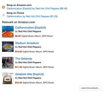
In Song Search when you've found a song, it loads some affiliate links to Amazon.com. (In case you're curious it's earning me lower double-digit dollars per month). To avoid overloading the Amazon Affiliate Product API, after I've queried their API, I store that result in my own database along with some metadata. Then, the next time someone views that song page, it can read from my local database. With me so far?
The other caveat is that you can't store these lookups locally too long since prices change and/or results change. So if my own stored result is older than a couple of hundred days, I delete it and fetch from the network again. My current implementation uses PostgreSQL (via the Django ORM) to store this stuff. The model looks like this:
classAmazonAffiliateLookup(models.Model,TotalCountMixin):song=models.ForeignKey(Song,on_delete=models.CASCADE)matches=JSONField(null=True)search_index=models.CharField(max_length=100,null=True)lookup_seconds=models.FloatField(null=True)created=models.DateTimeField(auto_now_add=True,db_index=True)modified=models.DateTimeField(auto_now=True)At the moment this database table is 3GB on disk.
Then, I thought, why not use Redis for this. Then I can use Redis's "natural" expiration by simply setting as expiry time when I store it and then I don't have to worry about cleaning up old stuff at all.
The way I'm using Redis in this project is as a/the cache backend and I have it configured like this:
CACHES={"default":{"BACKEND":"django_redis.cache.RedisCache","LOCATION":REDIS_URL,"TIMEOUT":config("CACHE_TIMEOUT",500),"KEY_PREFIX":config("CACHE_KEY_PREFIX",""),"OPTIONS":{"COMPRESSOR":"django_redis.compressors.zlib.ZlibCompressor","SERIALIZER":"django_redis.serializers.msgpack.MSGPackSerializer",},}}The speed difference
Perhaps unrealistic but I'm doing all this testing here on my MacBook Pro. The connection to Postgres (version 11.4) and Redis (3.2.1) are both on localhost.
Reads
The reads are the most important because hopefully, they happen 10x more than writes as several people can benefit from previous saves.
I changed my code so that it would do a read from both databases and if it was found in both, write down their time in a log file which I'll later summarize. Results are as follows:
PG:
median: 8.66ms
mean  : 11.18ms
stdev : 19.48ms

Redis:
median: 0.53ms
mean  : 0.84ms
stdev : 2.26ms

(310 measurements)
It means, when focussing on the median, Redis is 16 times faster than PostgreSQL at reading these JSON blobs.
Writes
The writes are less important but due to the synchronous nature of my Django, the unlucky user who triggers a look up that I didn't have, will have to wait for the write before the XHR request can be completed. However, when this happens, the remote network call to the Amazon Product API is bound to be much slower. Results are as follows:
PG:
median: 8.59ms
mean  : 8.58ms
stdev : 6.78ms

Redis:
median: 0.44ms
mean  : 0.49ms
stdev : 0.27ms

(137 measurements)
It means, when focussing on the median, Redis is 20 times faster than PostgreSQL at writing these JSON blobs.
Conclusion and discussion
First of all, I'm still a PostgreSQL fan-boy and have no intention of ceasing that. These times are made up of much more than just the individual databases. For example, the PostgreSQL speeds depend on the Django ORM code that makes the SQL and sends the query and then turns it into the model instance. I don't know what the proportions are between that and the actual bytes-from-PG's-disk times. But I'm not sure I care either. The tooling around the database is inevitable mostly and it's what matters to users.
Both Redis and PostgreSQL are persistent and survive server restarts and crashes etc. And you get so many more "batch related" features with PostgreSQL if you need them, such as being able to get a list of the last 10 rows added for some post-processing batch job.
I'm currently using Django's cache framework, with Redis as its backend, and it's a cache framework. It's not meant to be a persistent database. I like the idea that if I really have to I can just flush the cache and although detrimental to performance (temporarily) it shouldn't be a disaster. So I think what I'll do is store these JSON blobs in both databases. Yes, it means roughly 6GB of SSD storage but it also potentially means loading a LOT more into RAM on my limited server. That extra RAM usage pretty much sums of this whole blog post; of course it's faster if you can rely on RAM instead of disk. Now I just need to figure out how RAM I can afford myself for this piece and whether it's worth it.
↧
Weekly Python StackOverflow Report: (cxcvi) stackoverflow python report
These are the ten most rated questions at Stack Overflow last week.
Between brackets: [question score / answers count]
Build date: 2019-09-28 20:30:43 GMT
- Check reference list in pandas column using numpy vectorization - [7/3]
- Avoiding combination of pip and conda - [7/0]
- Does python reuse repeated calculation results? - [6/3]
- Numpy error when converting array of ctypes types to void pointer - [6/1]
- How to pass an intermediate amount of data to a subprocess? - [6/1]
- How to list all function names of a Python module in C++? - [6/1]
- Why does IPython manage memory differently than CPython when I delete a list? - [6/1]
- How to convert html `abbr` tag text to a text in parentheses in Python? - [5/2]
- How to count no of rows in a data frame whose values divisible by 3 or 5? - [5/2]
- Finding Power Using Recursion - [5/2]
↧
↧
Catalin George Festila: The tensorflow python module - part 004.
If you using the tensorflow then you can get some warnings.
You can use warnings python package to manage all of this:
[mythcat@desk ~]$ $ python3
Python 3.5.2 (default, Jul 10 2019, 11:58:48)
[GCC 5.4.0 20160609] on linux
Type "help", "copyright", "credits" or "license" for more information.
>>> import warnings
>>> import tensorflow as tf
/home/mythcat/.local/lib/python3.5/site-packages/
↧
Erik Marsja: How to use iloc and loc for Indexing and Slicing Pandas Dataframes
The post How to use iloc and loc for Indexing and Slicing Pandas Dataframes appeared first on Erik Marsja.
In this post, we are going to work with Pandas iloc, and loc. More specifically, we are going to learn slicing and indexing by iloc and loc examples.
Once we have a dataset loaded as a Pandas dataframe, we often want to start accessing specific parts of the data based on some criteria. For instance, if our dataset contains the result of an experiment comparing different experimental groups, we may want to calculate descriptive statistics for each experimental group separately.

The procedure of selecting specific rows and columns of data based on some criteria is commonly known as slicing.
Pandas Dataframes
Before we are going to learn how to work with loc and iloc, we are it can be good to have a reminder on how Pandas dataframe object work. For the specific purpose of this indexing and slicing tutorial it is good to know that each row and column, in the dataframe, has a number – an index.

This structure, a row-and-column structure with numeric indexes, means that we can work with data by using the row and the column numbers. This is useful to know when we are going to work with Pandas loc and iloc methods.
Data
In the following iloc and loc example we are going to work with two datasets. These datasets, among a lot of other RDatasets, can be found here but the following code will load them into Pandas dataframes:
import pandas as pd

url_dataset1 = 'https://vincentarelbundock.github.io/Rdatasets/csv/psych/affect.csv'
url_dataset2 = 'https://vincentarelbundock.github.io/Rdatasets/csv/DAAG/nasshead.csv'

df1 = pd.read_csv(url_dataset1, index_col=0)
df2 = pd.read_csv(url_dataset2, index_col=0)
If you are interested in learning more about in-and-out methods of Pandas make sure to check the following posts out:
- How to read CSV files in Pandas
- How to read Excel files in Pandas
- Reading SPSS files in Pandas
- Working with JSON files using Python and Pandas
What is the Difference Between loc and iloc?
Before going on and working with Pandas iloc and loc, we will answer the question concerning the difference between loc and iloc.
First of all, .loc is a label based method whereas .iloc is an integer based method. This means that iloc will consider the names or labels of the index when we are slicing for the dataframe.
For example, df2.loc[‘ case ‘] will result in all the third row being selected.

On the other hand, .iloc takes slices based on index’s position. Unlike .loc, .iloc behaves like regular Python slicing. That is, we just indicate the positional index number, and we get the slice we want.
For example, df1.iloc[2] will give us the third row of the dataframe. This is because, just like in Python, .iloc is zero positional based. That is it starts at 0. We will learn how we use loc and iloc, in the following sections of this post.
What does iloc do in Pandas?
As previously mentioned, Pandas iloc is primarily integer position based. That is, it can be used to index a dataframe using 0 to length-1 whether it’s the row or column indices.
Furthermore, as we will see in a later Pandas iloc example, the method can also be used with a boolean array.

In this Pandas iloc tutorial, we are going to work with the following input methods:
- An integer, e.g. 2
- A list of integers, e.g. [7, 2, 0]
- A slice object with ints, e.g. 0:7, as in the image above
- A boolean array.
How to use Pandas iloc
Now you may be wondering “how do I use iloc?” and we are, of course, going to answer that question. In the simplest form we just type an integer between the brackets.
df.iloc[0]
As can be seen in the Pandas iloc example, above, we typed a set of brackets after the iloc method.
Furthermore, we added an integer (0) as index value to specify that we wanted the first row of our dataframe. Now, here it’s important to know that order of the indexes inside the brackets obviously matters.
The first index number will be the row or rows that we want to retrieve. If we wat to retrieve a specific column, or specific columns, using iloc we input a second index (or indices). This, however, is optional and without a second index, iloc will retrieve all columns by default.
Pandas iloc syntax is, as previously described, DataFrame.iloc[<row selection>, <column selection>].

This may be confusing for users of R statistical programming environment. To iterate, the iloc method in Pandas is used to select rows and columns by number, in the order that they appear in the dataframe.
Pandas iloc Examples
In the next section, we continue this Pandas indexing and slicing tutorial by looking at different examples of how to use iloc. We have, of course, already started with the most basic one; selecting a single row:
df1.iloc[3]Indexing the last Row of a Pandas dataframe
In the next example, we are continuing using one integer to index the dataframe. However. if we want to retrieve the last row of a Pandas dataframe we use “-1”:
df1.iloc[-1]We can also input a list, with only one index integer, when we use iloc. This will index one row but the output will be different compared to the example above:
df1.iloc[[-1]]
Select Multiple Rows using iloc
We can, of course, also use iloc to select many rows from a pandas dataframe. For instance, if we add more index integers to the list, like in the example above, we can select many rows.
df.iloc[[7, 2, 0]]
Slicing Rows using iloc in Pandas
In the next Pandas iloc example, we are going to learn about slicing. Note, we are going to get more familiar using the slicing character “:” later in this post. To select row 11 to 15 we type the following code:
df1.iloc[10:15]
Selecting Columns with Pandas iloc
As previously indicated, we can, of course, when using the second argument in the iloc method also select, or slice, columns. In the next iloc example, we may want to retrieve the only the first column of the dataframe, which is the column at index position 0.
To do this, we will use an integer index value in the second position inside of the brackets when we use iloc. Note, the integer index in the second position specifies the column that we want to retrieve. What about the rows?

Note, that when we want to select all rows and one column (or many columns) using iloc we need to use the “:” character.
df1.iloc[:, 0]
In the Pandas iloc example above, we used the “:” character in the first position inside of the brackets. This indicates that we want to retrieve all the rows. A reminder; the first index position inside of [], specifies the rows, and the we used the “:” character, because we wanted to get all rows from a Pandas dataframe.
In the next example of how to use Pandas iloc, we are going to take a slice of the columns and all rows. This can be done in a similar way as above. However, instead of using a integer we use a Python slice to get all rows and the first 6 columns:
df1.iloc[:, 0:6]
Select a Specific Cell using iloc
In this section, of the Pandas iloc tutorial we will learn how to select a specific cell.
This is quite simple, of course, and we just use an integer index value for the row and for the column we want to get from the dataframe. For example, if we want to select the data in row 0 and column 0, we just type df1.iloc[0, 0].

Of course, we can also select multiple rows and/or multiple columns. To do this we just add a list with the integer indices that we want iloc to select for us.
For example, if we want to select the data in row 4 and column 2, 3, and 4 we just use the following code:
df1.iloc[3, [1, 2, 3]]Retrieving subsets of cells
In the next iloc example, we are going to get a subset of cells from the dataframe.
Acheiving this this is a combination of getting a slice of columns and a slice of rows with iloc:
df1.iloc[0:5, 3:7]Selecting Columns using a Boolean Mask
In the final example, we are going to select columns using a boolean mask. Doing this, of course require us to know how many columns there are and which columns we want to select.
bool_i = [False, False, True, True, True,
 True, True, True, True, True,
 True, True, True, True, True,
 True, True, True, False, False]

df.iloc[3:7, bool_i]
How to Use Pandas loc
In this section, we are covering another Pandas method, i.e. loc for selecting data from dataframes.

When to use loc?
Remember, whereas iloc takes the positional references as the argument input while loc takes indexes as the argument. As loc takes indexes, we can pass strings (e.g., column names) as an argument whereas it will throw an error if we used strings with iloc. So the answer to the question when to use Pandas loc? is when we know the index names.
In this loc tutorial we are going to use the following inputs:
- A single label, for instance 2 or ‘b’.
It is worth noting here that Pandas interpret 2 as a label of the index and not as an integer position along the index (contrary to iloc) - A list of labels, for instance [‘a’, ‘b’, c’]
- A slice object with labels, for example,. ‘shortname’:’SASname’. Importantly, when it comes to slices, when we use loc, BOTH the start and stop are included
Select a Row using Pandas loc
In the first Pandas loc example, we are going to select data from the row where the index is equal to 1.
df2.loc[1]Note, in the example above the first row has the name “1” . That is, this is not the index integer but the name.
Pandas loc behaves the in the same manner as iloc and we retrieve a single row as series. Just as with Pandas iloc, we can change the output so that it we get a single row as a dataframe. We do this by putting in the row name in a list:
df2.loc[[1]]
Slicing Rows using loc
In the next code example, we are going to take a slice of rows using the row names.
df2.loc[1:5]
We can also pass it a list of indexes to select required indexes.
df2.loc[[1, 6, 11, 21, 51]]
Selecting by Column Names using loc
Unlike Pandas iloc, loc futher takes column names as column argument. This means that we can pass it a column name to select data from that column.
In the next loc example, we are going to select all the data from the ‘SASname’ column.
df2.loc[:, 'SASname']Another option is, of course, to pass multiple column names in a list when using loc. In the next example, we are selecting data from the ‘SASname’, and ‘longname’ columns where the row names are from 1 to 5.
df2.loc[1:5, ['SASname', 'longname']]
Slicing using loc in Pandas
In this section, we will see how we can slice a Pandas dataframe using loc. Remember that the “:” character is used when slicing. As with iloc, we can also slice but here we can column names and row names (like in the example below).
In the loc example below, we use the first dataframe again (df1, that is) and slice the first 5 rows and take the columns from the ‘Film’ column to the ‘EA1’ column
df1.loc[1:5, 'Film':'EA1']Pandas iloc and Conditions
Many times we want to index a Pandas dataframe by using boolean arrays. That is, we may want to select data based on certain conditions. This is quite easy to do with Pandas loc, of course. We just pass an array or Seris of True/False values to the .loc method.
For example, if we want select all rows where the value in the Study column is “flat” we do as follows to create a Pandas Series with a True value for every row in the dataframe, where “flat” exists.
df1.loc[df1['Study'] == 'flat']
Select Rows using Multiple Conditions Pandas iloc
Furthermore, some times we may want to select based on more than one condition. For instance, if we want to select all rows here the value in the Study column is “flat” and and the value in the neur column is larger than 18 we do as in the next example:
df1.loc[(df1['neur'] > 18) & (df1['Study'] == 'flat')]
As before, we can use a second to select particular columns out of the dataframe. Remember, when working with Pandas loc, columns are referred to by name for the loc indexer and we can use a single string, a list of columns, or a slice “:” operation. In the next example, we select the columns from EA1 to NA2:
df1.loc[(df1['neur'] > 18) & (df1['Study'] == 'flat'), 'EA1':'NA2']
Setting Values in dataframes using .loc
In the last section, of this loc and iloc tutorial, we are going to learn how to set values to the dataframe using loc.
Setting values to a dataframe is easy all we need is to change the syntax a bit, and we can actually update the data in the same statement as weselect and filter using .loc indexer. This is handy as we can to update values in columns depending on different conditions.
In the final loc example, we are going to create a new coumn (NewCol) and add the word “BIG” there in the rows where neur is larger than 18:
df1.loc[df1['neur'] > 18, 'NewCol'] = 'BIG'
df1.loc[df1['neur'] > 18, 'EA1':'NewCol'].head()
Conclusion
In this Pandas iloc and loc tutorial we have learned indexing, selecting, and subsetting using the loc and iloc methods. More specifically, we have learned how these to methods work. When it comes to loc we have learned how to select based on conditional statements (e.g., larger than or equal to) as well as that we have learned how to set values using loc.
The post How to use iloc and loc for Indexing and Slicing Pandas Dataframes appeared first on Erik Marsja.
↧
Peter Bengtsson: Update to speed comparison for Redis vs PostgreSQL storing blobs of JSON
Last week, I blogged about "How much faster is Redis at storing a blob of JSON compared to PostgreSQL?". Judging from a lot of comments, people misinterpreted this. (By the way, Redis is persistent). It's no surprise that Redis is faster.
However, it's a fact that I have do have a lot of blobs stored and need to present them via the web API as fast as possible. It's rare that I want to do relational or batch operations on the data. But Redis isn't a slam dunk for simple retrieval because I don't know if I trust its integrity with the 3GB worth of data that I both don't want to lose and don't want to load all into RAM.
But is it entirely wrong to look at WHICH database to get the best speed?
Reviewing this corner of Song Search helped me rethink this. PostgreSQL is, in my view, a better database for storing stuff. Redis is faster for individual lookups. But you know what's even faster? Nginx
Nginx??
The way the application works is that a React web app is requesting the Amazon product data for the sake of presenting an appropriate affiliate link. This is done by the browser essentially doing:
constresponse=awaitfetch('https://songsear.ch/api/song/5246889/amazon');Internally, in the app, what it does is that it looks this up, by ID, on the AmazonAffiliateLookup ORM model. Suppose it wasn't there in the PostgreSQL, it uses the Amazon Affiliate Product Details API, to look it up and when the results come in it stores a copy of this in PostgreSQL so we can re-use this URL without hitting rate limits on the Product Details API. Lastly, in a piece of Django view code, it carefully scrubs and repackages this result so that only the fields used by the React rendering code is shipped between the server and the browser. That "scrubbed" piece of data is actually much smaller. Partly because it limits the results to the first/best match and it deletes a bunch of things that are never needed such as ProductTypeName, Studio, TrackSequence etc. The proportion is roughly 23x. I.e. of the 3GB of JSON blobs stored in PostgreSQL only 130MB is ever transported from the server to the users.
Again, Nginx?
Nginx has a built in reverse HTTP proxy cache which is easy to set up but a bit hard to do purges on. The biggest flaw, in my view, is that it's hard to get a handle of how much RAM this it's eating up. Well, if the total possible amount of data within the server is 130MB, then that is something I'm perfectly comfortable to let Nginx handle cache in RAM.
Good HTTP performance benchmarking is hard to do but here's a teaser from my local laptop version of Nginx:
▶ hey -n 10000 -c 10 https://songsearch.local/api/song/1810960/affiliate/amazon-itunes

Summary:
  Total:    0.9882 secs
  Slowest:  0.0279 secs
  Fastest:  0.0001 secs
  Average:  0.0010 secs
  Requests/sec: 10119.8265


Response time histogram:
  0.000 [1] |
  0.003 [9752]  |■■■■■■■■■■■■■■■■■■■■■■■■■■■■■■■■■■■■■■■■
  0.006 [108]   |
  0.008 [70]    |
  0.011 [32]    |
  0.014 [8] |
  0.017 [12]    |
  0.020 [11]    |
  0.022 [1] |
  0.025 [4] |
  0.028 [1] |


Latency distribution:
  10% in 0.0003 secs
  25% in 0.0006 secs
  50% in 0.0008 secs
  75% in 0.0010 secs
  90% in 0.0013 secs
  95% in 0.0016 secs
  99% in 0.0068 secs

Details (average, fastest, slowest):
  DNS+dialup:   0.0000 secs, 0.0001 secs, 0.0279 secs
  DNS-lookup:   0.0000 secs, 0.0000 secs, 0.0026 secs
  req write:    0.0000 secs, 0.0000 secs, 0.0011 secs
  resp wait:    0.0008 secs, 0.0001 secs, 0.0206 secs
  resp read:    0.0001 secs, 0.0000 secs, 0.0013 secs

Status code distribution:
  [200] 10000 responses
10,000 requests across 10 clients at rougly 10,000 requests per second. That includes doing all the HTTP parsing, WSGI stuff, forming of a SQL or Redis query, the deserialization, the Django JSON HTTP response serialization etc. The cache TTL is controlled by simply setting a Cache-Control HTTP header with something like max-age=86400.
Now, repeated fetches for this are cached at the Nginx level and it means it doesn't even matter how slow/fast the database is. As long as it's not taking seconds, with a long Cache-Control, Nginx can hold on to this in RAM for days or until the whole server is restarted (which is rare).
Conclusion
If you the total amount of data that can and will be cached is controlled, putting it in a HTTP reverse proxy cache is probably order of magnitude faster than messing with chosing which database to use.
↧