Are there certain parts of Python that just seem magic? Like how are dictionaries so much faster than looping over a list to find an item. How does a generator remember the state of the variables each time it yields a value and why do you never have to allocate memory like other languages? It turns out, CPython, the most popular Python runtime is written in human-readable C and Python code. This tutorial will walk you through the CPython source code.
You’ll cover all the concepts behind the internals of CPython, how they work and visual explanations as you go.
You’ll learn how to:
- Read and navigate the source code
- Compile CPython from source code
- Navigate and comprehend the inner workings of concepts like lists, dictionaries, and generators
- Run the test suite
- Modify or upgrade components of the CPython library to contribute them to future versions
Yes, this is a very long article. If you just made yourself a fresh cup of tea, coffee or your favorite beverage, it’s going to be cold by the end of Part 1.
This tutorial is split into five parts. Take your time for each part and make sure you try out the demos and the interactive components. You can feel a sense of achievement that you grasp the core concepts of Python that can make you a better Python programmer.
Free Bonus:5 Thoughts On Python Mastery, a free course for Python developers that shows you the roadmap and the mindset you'll need to take your Python skills to the next level.
Part 1: Introduction to CPython
When you type python at the console or install a Python distribution from python.org, you are running CPython. CPython is one of the many Python runtimes, maintained and written by different teams of developers. Some other runtimes you may have heard are PyPy, Cython, and Jython.
The unique thing about CPython is that it contains both a runtime and the shared language specification that all Python runtimes use. CPython is the “official,” or reference implementation of Python.
The Python language specification is the document that the description of the Python language. For example, it says that assert is a reserved keyword, and that [] is used for indexing, slicing, and creating empty lists.
Think about what you expect to be inside the Python distribution on your computer:
- When you type
python without a file or module, it gives an interactive prompt. - You can import built-in modules from the standard library like
json. - You can install packages from the internet using
pip. - You can test your applications using the built-in
unittest library.
These are all part of the CPython distribution. There’s a lot more than just a compiler.
Note: This article is written against version 3.8.0b3 of the CPython source code.
What’s in the Source Code?
The CPython source distribution comes with a whole range of tools, libraries, and components. We’ll explore those in this article. First we are going to focus on the compiler.
To download a copy of the CPython source code, you can use git to pull the latest version to a working copy locally:
git clone https://github.com/python/cpython
Note: If you don’t have Git available, you can download the source in a ZIP file directly from the GitHub website.
Inside of the newly downloaded cpython directory, you will find the following subdirectories:
cpython/
│
├── Doc      ← Source for the documentation
├── Grammar  ← The a computer-readable language definition
├── Include  ← The C header files
├── Lib      ← Standard library modules written in Python
├── Mac      ← macOS support files
├── Misc     ← Miscellaneous files
├── Modules  ← Standard Library Modules written in C
├── Objects  ← Core types and the object model
├── Parser   ← The Python parser source code
├── PC       ← Windows build support files
├── PCbuild  ← Windows build support files for older Windows versions
├── Programs ← Source code for the python executable and other binaries
├── Python   ← The CPython interpreter source code
└── Tools    ← Standalone tools useful for building or extending Python
Next, we’ll compile CPython from the source code. This step requires a C compiler, and some build tools, which depend on the operating system you’re using.
Compiling CPython (macOS)
Compiling CPython on macOS is straightforward. You will first need the essential C compiler toolkit. The Command Line Development Tools is an app that you can update in macOS through the App Store. You need to perform the initial installation on the terminal.
To open up a terminal in macOS, go to the Launchpad, then Other then choose the Terminal app. You will want to save this app to your Dock, so right-click the Icon and select Keep in Dock.
Now, within the terminal, install the C compiler and toolkit by running the following:
This command will pop up with a prompt to download and install a set of tools, including Git, Make, and the GNU C compiler.
You will also need a working copy of OpenSSL to use for fetching packages from the PyPi.org website. If you later plan on using this build to install additional packages, SSL validation is required.
The simplest way to install OpenSSL on macOS is by using HomeBrew. If you already have HomeBrew installed, you can install the dependencies for CPython with the brew install command:
$ brew install openssl xz zlib
Now that you have the dependencies, you can run the configure script, enabling SSL support by discovering the location that HomeBrew installed to and enabling the debug hooks --with-pydebug:
$CPPFLAGS="-I$(brew --prefix zlib)/include"\LDFLAGS="-L$(brew --prefix zlib)/lib"\
 ./configure --with-openssl=$(brew --prefix openssl) --with-pydebug
This will generate a Makefile in the root of the repository that you can use to automate the build process. The ./configure step only needs to be run once. You can build the CPython binary by running:
The -j2 flag allows make to run 2 jobs simultaneously. If you have 4 cores, you can change this to 4. The -s flag stops the Makefile from printing every command it runs to the console. You can remove this, but the output is very verbose.
During the build, you may receive some errors, and in the summary, it will notify you that not all packages could be built. For example, _dbm, _sqlite3, _uuid, nis, ossaudiodev, spwd, and _tkinter would fail to build with this set of instructions. That’s okay if you aren’t planning on developing against those packages. If you are, then check out the dev guide website for more information.
The build will take a few minutes and generate a binary called python.exe. Every time you make changes to the source code, you will need to re-run make with the same flags.
The python.exe binary is the debug binary of CPython. Execute python.exe to see a working REPL:
$ ./python.exe
Python 3.8.0b3 (tags/v3.8.0b3:4336222407, Aug 21 2019, 10:00:03) [Clang 10.0.1 (clang-1001.0.46.4)] on darwinType "help", "copyright", "credits" or "license" for more information.>>>
Note:
Yes, that’s right, the macOS build has a file extension for .exe. This is not because it’s a Windows binary. Because macOS has a case-insensitive filesystem and when working with the binary, the developers didn’t want people to accidentally refer to the directory Python/ so .exe was appended to avoid ambiguity.
If you later run make install or make altinstall, it will rename the file back to python.
Compiling CPython (Linux)
For Linux, the first step is to download and install make, gcc, configure, and pkgconfig.
For Fedora Core, RHEL, CentOS, or other yum-based systems:
$ sudo yum install yum-utils
For Debian, Ubuntu, or other apt-based systems:
$ sudo apt install build-essential
Then install the required packages, for Fedora Core, RHEL, CentOS or other yum-based systems:
$ sudo yum-builddep python3
For Debian, Ubuntu, or other apt-based systems:
$ sudo apt install libssl-dev zlib1g-dev libncurses5-dev \
  libncursesw5-dev libreadline-dev libsqlite3-dev libgdbm-dev \
  libdb5.3-dev libbz2-dev libexpat1-dev liblzma-dev libffi-dev
Now that you have the dependencies, you can run the configure script, enabling the debug hooks --with-pydebug:
$ ./configure --with-pydebug
Review the output to ensure that OpenSSL support was marked as YES. Otherwise, check with your distribution for instructions on installing the headers for OpenSSL.
Next, you can build the CPython binary by running the generated Makefile:
During the build, you may receive some errors, and in the summary, it will notify you that not all packages could be built. That’s okay if you aren’t planning on developing against those packages. If you are, then check out the dev guide website for more information.
The build will take a few minutes and generate a binary called python. This is the debug binary of CPython. Execute ./python to see a working REPL:
$ ./python
Python 3.8.0b3 (tags/v3.8.0b3:4336222407, Aug 21 2019, 10:00:03) [Clang 10.0.1 (clang-1001.0.46.4)] on darwinType "help", "copyright", "credits" or "license" for more information.>>>
Compiling CPython (Windows)
Inside the PC folder is a Visual Studio project file for building and exploring CPython. To use this, you need to have Visual Studio installed on your PC.
The newest version of Visual Studio, Visual Studio 2019, makes it easier to work with Python and the CPython source code, so it is recommended for use in this tutorial. If you already have Visual Studio 2017 installed, that would also work fine.
None of the paid features are required for compiling CPython or this tutorial. You can use the Community edition of Visual Studio, which is available for free from Microsoft’s Visual Studio website.
Once you’ve downloaded the installer, you’ll be asked to select which components you want to install. The bare minimum for this tutorial is:
- The Python Development workload
- The optional Python native development tools
- Python 3 64-bit (3.7.2) (can be deselected if you already have Python 3.7 installed)
Any other optional features can be deselected if you want to be more conscientious with disk space:
![Visual Studio Options Window]()
The installer will then download and install all of the required components. The installation could take an hour, so you may want to read on and come back to this section.
Once the installer has completed, click the Launch button to start Visual Studio. You will be prompted to sign in. If you have a Microsoft account you can log in, or skip that step.
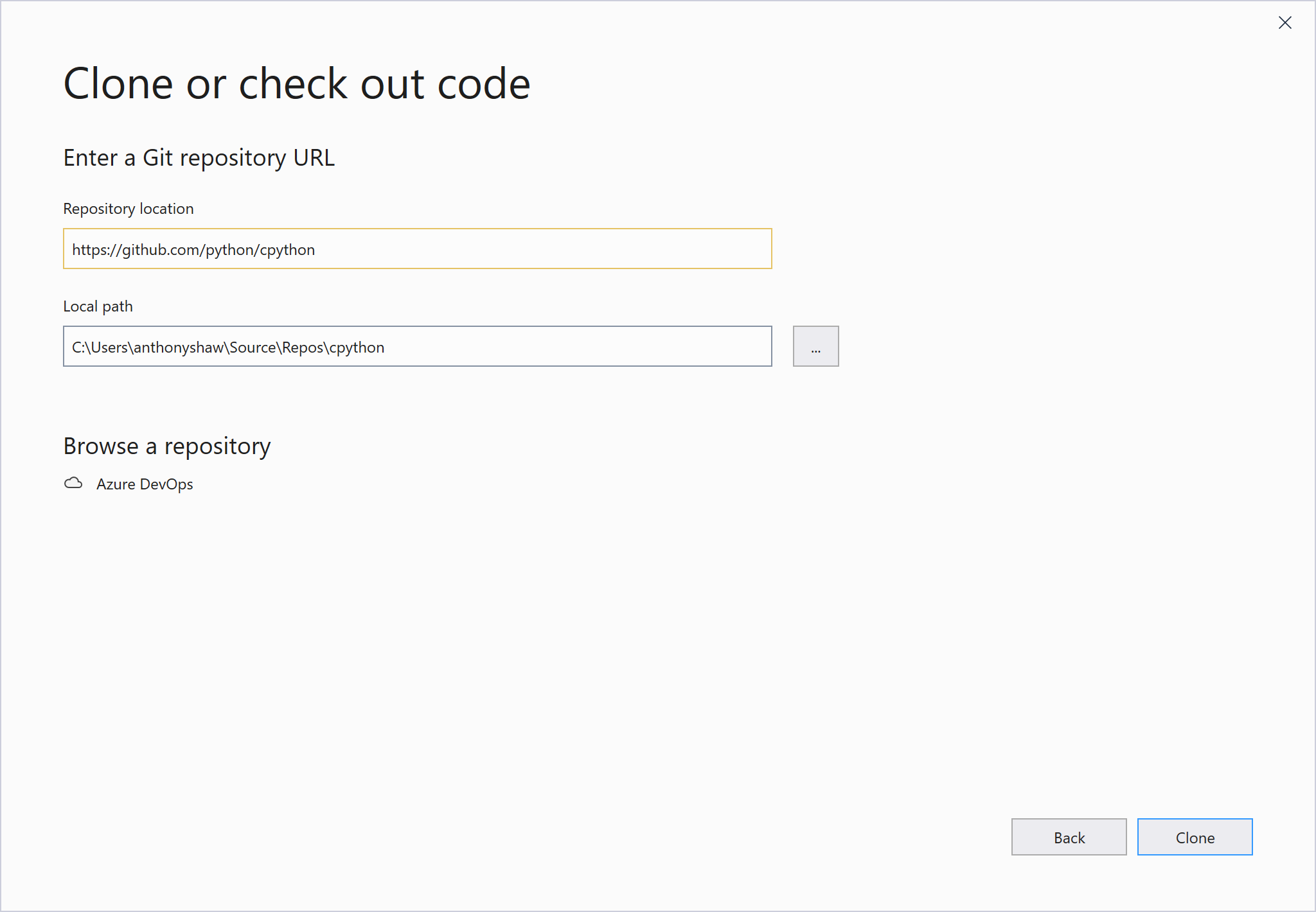
Once Visual Studio starts, you will be prompted to Open a Project. A shortcut to getting started with the Git configuration and cloning CPython is to choose the Clone or check out code option:
![Choosing a Project Type in Visual Studio]()
For the project URL, type https://github.com/python/cpython to clone:
![Cloning projects in Visual Studio]()
Visual Studio will then download a copy of CPython from GitHub using the version of Git bundled with Visual Studio. This step also saves you the hassle of having to install Git on Windows. The download may take 10 minutes.
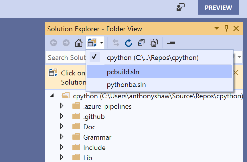
Once the project has downloaded, you need to point it to the pcbuild Solution file, by clicking on Solutions and Projects and selecting pcbuild.sln:
![Selecting a solution]()
When the solution is loaded, it will prompt you to retarget the project’s inside the solution to the version of the C/C++ compiler you have installed. Visual Studio will also target the version of the Windows SDK you have installed.
Ensure that you change the Windows SDK version to the newest installed version and the platform toolset to the latest version. If you missed this window, you can right-click on the Solution in the Solutions and Projects window and click Retarget Solution.
Once this is complete, you need to download some source files to be able to build the whole CPython package. Inside the PCBuild folder there is a .bat file that automates this for you. Open up a command-line prompt inside the downloaded PCBuild and run get_externals.bat:
> get_externals.batUsing py -3.7 (found 3.7 with py.exe)Fetching external libraries...Fetching bzip2-1.0.6...Fetching sqlite-3.21.0.0...Fetching xz-5.2.2...Fetching zlib-1.2.11...Fetching external binaries...Fetching openssl-bin-1.1.0j...Fetching tcltk-8.6.9.0...Finished.
Next, back within Visual Studio, build CPython by pressing Ctrl+Shift+B, or choosing Build Solution from the top menu. If you receive any errors about the Windows SDK being missing, make sure you set the right targeting settings in the Retarget Solution window. You should also see Windows Kits inside your Start Menu, and Windows Software Development Kit inside of that menu.
The build stage could take 10 minutes or more for the first time. Once the build is completed, you may see a few warnings that you can ignore and eventual completion.
To start the debug version of CPython, press F5 and CPython will start in Debug mode straight into the REPL:
![CPython debugging Windows]()
Once this is completed, you can run the Release build by changing the build configuration from Debug to Release on the top menu bar and rerunning Build Solution again.
You now have both Debug and Release versions of the CPython binary within PCBuild\win32\.
You can set up Visual Studio to be able to open a REPL with either the Release or Debug build by choosing Tools->Python->Python Environments from the top menu:
![Choosing Python environments]()
Then click Add Environment and then target the Debug or Release binary. The Debug binary will end in _d.exe, for example, python_d.exe and pythonw_d.exe. You will most likely want to use the debug binary as it comes with Debugging support in Visual Studio and will be useful for this tutorial.
In the Add Environment window, target the python_d.exe file as the interpreter inside the PCBuild/win32 and the pythonw_d.exe as the windowed interpreter:
![Adding an environment in VS2019]()
Now, you can start a REPL session by clicking Open Interactive Window in the Python Environments window and you will see the REPL for the compiled version of Python:
![Python Environment REPL]()
During this tutorial there will be REPL sessions with example commands. I encourage you to use the Debug binary to run these REPL sessions in case you want to put in any breakpoints within the code.
Lastly, to make it easier to navigate the code, in the Solution View, click on the toggle button next to the Home icon to switch to Folder view:
![Switching Environment Mode]()
Now you have a version of CPython compiled and ready to go, let’s find out how the CPython compiler works.
What Does a Compiler Do?
The purpose of a compiler is to convert one language into another. Think of a compiler like a translator. You would hire a translator to listen to you speaking in English and then speak in Japanese:
![Translating from English to Japanese]()
Some compilers will compile into a low-level machine code which can be executed directly on a system. Other compilers will compile into an intermediary language, to be executed by a virtual machine.
One important decision to make when choosing a compiler is the system portability requirements. Java and .NET CLR will compile into an Intermediary Language so that the compiled code is portable across multiple systems architectures. C, Go, C++, and Pascal will compile into a low-level executable that will only work on systems similar to the one it was compiled.
Because Python applications are typically distributed as source code, the role of the Python runtime is to convert the Python source code and execute it in one step. Internally, the CPython runtime does compile your code. A popular misconception is that Python is an interpreted language. It is actually compiled.
Python code is not compiled into machine-code. It is compiled into a special low-level intermediary language called bytecode that only CPython understands. This code is stored in .pyc files in a hidden directory and cached for execution. If you run the same Python application twice without changing the source code, it’ll always be much faster the second time. This is because it loads the compiled bytecode and executes it directly.
Why Is CPython Written in C and Not Python?
The C in CPython is a reference to the C programming language, implying that this Python distribution is written in the C language.
This statement is largely true: the compiler in CPython is written in pure C. However, many of the standard library modules are written in pure Python or a combination of C and Python.
So why is CPython written in C and not Python?
The answer is located in how compilers work. There are two types of compiler:
- Self-hosted compilers are compilers written in the language they compile, such as the Go compiler.
- Source-to-source compilers are compilers written in another language that already have a compiler.
If you’re writing a new programming language from scratch, you need an executable application to compile your compiler! You need a compiler to execute anything, so when new languages are developed, they’re often written first in an older, more established language.
A good example would be the Go programming language. The first Go compiler was written in C, then once Go could be compiled, the compiler was rewritten in Go.
CPython kept its C heritage: many of the standard library modules, like the ssl module or the sockets module, are written in C to access low-level operating system APIs.
The APIs in the Windows and Linux kernels for creating network sockets, working with the filesystem or interacting with the display are all written in C. It made sense for Python’s extensibility layer to be focused on the C language. Later in this article, we will cover the Python Standard Library and the C modules.
There is a Python compiler written in Python called PyPy. PyPy’s logo is an Ouroboros to represent the self-hosting nature of the compiler.
Another example of a cross-compiler for Python is Jython. Jython is written in Java and compiles from Python source code into Java bytecode. In the same way that CPython makes it easy to import C libraries and use them from Python, Jython makes it easy to import and reference Java modules and classes.
The Python Language Specification
Contained within the CPython source code is the definition of the Python language. This is the reference specification used by all the Python interpreters.
The specification is in both human-readable and machine-readable format. Inside the documentation is a detailed explanation of the Python language, what is allowed, and how each statement should behave.
Documentation
Located inside the Doc/reference directory are reStructuredText explanations of each of the features in the Python language. This forms the official Python reference guide on docs.python.org.
Inside the directory are the files you need to understand the whole language, structure, and keywords:
cpython/Doc/reference
|
├── compound_stmts.rst
├── datamodel.rst
├── executionmodel.rst
├── expressions.rst
├── grammar.rst
├── import.rst
├── index.rst
├── introduction.rst
├── lexical_analysis.rst
├── simple_stmts.rst
└── toplevel_components.rst
Inside compound_stmts.rst, the documentation for compound statements, you can see a simple example defining the with statement.
The with statement can be used in multiple ways in Python, the simplest being the instantiation of a context-manager and a nested block of code:
You can assign the result to a variable using the as keyword:
You can also chain context managers together with a comma:
Next, we’ll explore the computer-readable documentation of the Python language.
Grammar
The documentation contains the human-readable specification of the language, and the machine-readable specification is housed in a single file, Grammar/Grammar.
The Grammar file is written in a context-notation called Backus-Naur Form (BNF). BNF is not specific to Python and is often used as the notation for grammars in many other languages.
The concept of grammatical structure in a programming language is inspired by Noam Chomsky’s work on Syntactic Structures in the 1950s!
Python’s grammar file uses the Extended-BNF (EBNF) specification with regular-expression syntax. So, in the grammar file you can use:
* for repetition+ for at-least-once repetition[] for optional parts| for alternatives() for grouping
If you search for the with statement in the grammar file, at around line 80 you’ll see the definitions for the with statement:
with_stmt: 'with' with_item (',' with_item)*  ':' suite
with_item: test ['as' expr]
Anything in quotes is a string literal, which is how keywords are defined. So the with_stmt is specified as:
- Starting with the word
with - Followed by a
with_item, which is a test and (optionally), the word as, and an expression - Following one or many items, each separated by a comma
- Ending with a
: - Followed by a
suite
There are references to some other definitions in these two lines:
suite refers to a block of code with one or multiple statementstest refers to a simple statement that is evaluatedexpr refers to a simple expression
If you want to explore those in detail, the whole of the Python grammar is defined in this single file.
If you want to see a recent example of how grammar is used, in PEP 572 the colon equals operator was added to the grammar file in this Git commit.
Using pgen
The grammar file itself is never used by the Python compiler. Instead, a parser table created by a tool called pgen is used. pgen reads the grammar file and converts it into a parser table. If you make changes to the grammar file, you must regenerate the parser table and recompile Python.
Note: The pgen application was rewritten in Python 3.8 from C to pure Python.
To see pgen in action, let’s change part of the Python grammar. Around line 51 you will see the definition of a pass statement:
Change that line to accept the keyword 'pass' or 'proceed' as keywords:
pass_stmt: 'pass' | 'proceed'
Now you need to rebuild the grammar files.
On macOS and Linux, run make regen-grammar to run pgen over the altered grammar file. For Windows, there is no officially supported way of running pgen. However, you can clone my fork and run build.bat --regen from within the PCBuild directory.
You should see an output similar to this, showing that the new Include/graminit.h and Python/graminit.c files have been generated:
# Regenerate Doc/library/token-list.inc from Grammar/Tokens
# using Tools/scripts/generate_token.py
...
python3 ./Tools/scripts/update_file.py ./Include/graminit.h ./Include/graminit.h.new
python3 ./Tools/scripts/update_file.py ./Python/graminit.c ./Python/graminit.c.new
With the regenerated parser tables, you need to recompile CPython to see the new syntax. Use the same compilation steps you used earlier for your operating system.
If the code compiled successfully, you can execute your new CPython binary and start a REPL.
In the REPL, you can now try defining a function and instead of using the pass statement, use the proceed keyword alternative that you compiled into the Python grammar:
Python 3.8.0b3 (tags/v3.8.0b3:4336222407, Aug 21 2019, 10:00:03)
[Clang 10.0.1 (clang-1001.0.46.4)] on darwin
Type "help", "copyright", "credits" or "license" for more information.
>>> def example():
...    proceed
...
>>> example()
Well done! You’ve changed the CPython syntax and compiled your own version of CPython. Ship it!
Next, we’ll explore tokens and their relationship to grammar.
Tokens
Alongside the grammar file in the Grammar folder is a Tokens file, which contains each of the unique types found as a leaf node in a parse tree. We will cover parser trees in depth later.
Each token also has a name and a generated unique ID. The names are used to make it simpler to refer to in the tokenizer.
Note: The Tokens file is a new feature in Python 3.8.
For example, the left parenthesis is called LPAR, and semicolons are called SEMI. You’ll see these tokens later in the article:
LPAR                    '('
RPAR                    ')'
LSQB                    '['
RSQB                    ']'
COLON                   ':'
COMMA                   ','
SEMI                    ';'
As with the Grammar file, if you change the Tokens file, you need to run pgen again.
To see tokens in action, you can use the tokenize module in CPython. Create a simple Python script called test_tokens.py:
# Hello world!defmy_function():proceed
For the rest of this tutorial, ./python.exe will refer to the compiled version of CPython. However, the actual command will depend on your system.
For Windows:
For Linux:
For macOS:
Then pass this file through a module built into the standard library called tokenize. You will see the list of tokens, by line and character. Use the -e flag to output the exact token name:
$ ./python.exe -m tokenize -e test_tokens.py

0,0-0,0:            ENCODING       'utf-8'        1,0-1,14:           COMMENT        '# Hello world!'1,14-1,15:          NL             '\n'           2,0-2,3:            NAME           'def'          2,4-2,15:           NAME           'my_function'  2,15-2,16:          LPAR           '('            2,16-2,17:          RPAR           ')'            2,17-2,18:          COLON          ':'            2,18-2,19:          NEWLINE        '\n'           3,0-3,3:            INDENT         '   '          3,3-3,7:            NAME           'proceed'         3,7-3,8:            NEWLINE        '\n'           4,0-4,0:            DEDENT         ''             4,0-4,0:            ENDMARKER      ''
In the output, the first column is the range of the line/column coordinates, the second column is the name of the token, and the final column is the value of the token.
In the output, the tokenize module has implied some tokens that were not in the file. The ENCODING token for utf-8, and a blank line at the end, giving DEDENT to close the function declaration and an ENDMARKER to end the file.
It is best practice to have a blank line at the end of your Python source files. If you omit it, CPython adds it for you, with a tiny performance penalty.
The tokenize module is written in pure Python and is located in Lib/tokenize.py within the CPython source code.
Important: There are two tokenizers in the CPython source code: one written in Python, demonstrated here, and another written in C.
The tokenizer written in Python is meant as a utility, and the one written in C is used by the Python compiler. They have identical output and behavior. The version written in C is designed for performance and the module in Python is designed for debugging.
To see a verbose readout of the C tokenizer, you can run Python with the -d flag. Using the test_tokens.py script you created earlier, run it with the following:
$ ./python.exe -d test_tokens.py

Token NAME/'def' ... It's a keyword DFA 'file_input', state 0: Push 'stmt' DFA 'stmt', state 0: Push 'compound_stmt' DFA 'compound_stmt', state 0: Push 'funcdef' DFA 'funcdef', state 0: Shift.Token NAME/'my_function' ... It's a token we know DFA 'funcdef', state 1: Shift.Token LPAR/'(' ... It's a token we know DFA 'funcdef', state 2: Push 'parameters' DFA 'parameters', state 0: Shift.Token RPAR/')' ... It's a token we know DFA 'parameters', state 1: Shift.  DFA 'parameters', state 2: Direct pop.Token COLON/':' ... It's a token we know DFA 'funcdef', state 3: Shift.Token NEWLINE/'' ... It's a token we know DFA 'funcdef', state 5: [switch func_body_suite to suite] Push 'suite' DFA 'suite', state 0: Shift.Token INDENT/'' ... It's a token we know DFA 'suite', state 1: Shift.Token NAME/'proceed' ... It's a keyword DFA 'suite', state 3: Push 'stmt'...  ACCEPT.
In the output, you can see that it highlighted proceed as a keyword. In the next chapter, we’ll see how executing the Python binary gets to the tokenizer and what happens from there to execute your code.
Now that you have an overview of the Python grammar and the relationship between tokens and statements, there is a way to convert the pgen output into an interactive graph.
Here is a screenshot of the Python 3.8a2 grammar:
![Python 3.8 DFA node graph]()
The Python package used to generate this graph, instaviz, will be covered in a later chapter.
Memory Management in CPython
Throughout this article, you will see references to a PyArena object. The arena is one of CPython’s memory management structures. The code is within Python/pyarena.c and contains a wrapper around C’s memory allocation and deallocation functions.
In a traditionally written C program, the developer should allocate memory for data structures before writing into that data. This allocation marks the memory as belonging to the process with the operating system.
It is also up to the developer to deallocate, or “free,” the allocated memory when its no longer being used and return it to the operating system’s block table of free memory.
If a process allocates memory for a variable, say within a function or loop, when that function has completed, the memory is not automatically given back to the operating system in C. So if it hasn’t been explicitly deallocated in the C code, it causes a memory leak. The process will continue to take more memory each time that function runs until eventually, the system runs out of memory, and crashes!
Python takes that responsibility away from the programmer and uses two algorithms: a reference counter and a garbage collector.
Whenever an interpreter is instantiated, a PyArena is created and attached one of the fields in the interpreter. During the lifecycle of a CPython interpreter, many arenas could be allocated. They are connected with a linked list. The arena stores a list of pointers to Python Objects as a PyListObject. Whenever a new Python object is created, a pointer to it is added using PyArena_AddPyObject(). This function call stores a pointer in the arena’s list, a_objects.
The PyArena serves a second function, which is to allocate and reference a list of raw memory blocks. For example, a PyList would need extra memory if you added thousands of additional values. The PyList object’s C code does not allocate memory directly. The object gets raw blocks of memory from the PyArena by calling PyArena_Malloc() from the PyObject with the required memory size. This task is completed by another abstraction in Objects/oballoc.c. In the object allocation module, memory can be allocated, freed, and reallocated for a Python Object.
A linked list of allocated blocks is stored inside the arena, so that when an interpreter is stopped, all managed memory blocks can be deallocated in one go using PyArena_Free().
Take the PyListObject example. If you were to .append() an object to the end of a Python list, you don’t need to reallocate the memory used in the existing list beforehand. The .append() method calls list_resize() which handles memory allocation for lists. Each list object keeps a list of the amount of memory allocated. If the item you’re appending will fit inside the existing free memory, it is simply added. If the list needs more memory space, it is expanded. Lists are expanded in length as 0, 4, 8, 16, 25, 35, 46, 58, 72, 88.
PyMem_Realloc() is called to expand the memory allocated in a list. PyMem_Realloc() is an API wrapper for pymalloc_realloc().
Python also has a special wrapper for the C call malloc(), which sets the max size of the memory allocation to help prevent buffer overflow errors (See PyMem_RawMalloc()).
In summary:
- Allocation of raw memory blocks is done via
PyMem_RawAlloc(). - The pointers to Python objects are stored within the
PyArena. PyArena also stores a linked-list of allocated memory blocks.
More information on the API is detailed on the CPython documentation.
Reference Counting
To create a variable in Python, you have to assign a value to a uniquely named variable:
Whenever a value is assigned to a variable in Python, the name of the variable is checked within the locals and globals scope to see if it already exists.
Because my_variable is not already within the locals() or globals() dictionary, this new object is created, and the value is assigned as being the numeric constant 180392.
There is now one reference to my_variable, so the reference counter for my_variable is incremented by 1.
You will see function calls Py_INCREF() and Py_DECREF() throughout the C source code for CPython. These functions increment and decrement the count of references to that object.
References to an object are decremented when a variable falls outside of the scope in which it was declared. Scope in Python can refer to a function or method, a comprehension, or a lambda function. These are some of the more literal scopes, but there are many other implicit scopes, like passing variables to a function call.
The handling of incrementing and decrementing references based on the language is built into the CPython compiler and the core execution loop, ceval.c, which we will cover in detail later in this article.
Whenever Py_DECREF() is called, and the counter becomes 0, the PyObject_Free() function is called. For that object PyArena_Free() is called for all of the memory that was allocated.
Garbage Collection
How often does your garbage get collected? Weekly, or fortnightly?
When you’re finished with something, you discard it and throw it in the trash. But that trash won’t get collected straight away. You need to wait for the garbage trucks to come and pick it up.
CPython has the same principle, using a garbage collection algorithm. CPython’s garbage collector is enabled by default, happens in the background and works to deallocate memory that’s been used for objects which are no longer in use.
Because the garbage collection algorithm is a lot more complex than the reference counter, it doesn’t happen all the time, otherwise, it would consume a huge amount of CPU resources. It happens periodically, after a set number of operations.
CPython’s standard library comes with a Python module to interface with the arena and the garbage collector, the gc module. Here’s how to use the gc module in debug mode:
>>>>>> importgc>>> gc.set_debug(gc.DEBUG_STATS)
This will print the statistics whenever the garbage collector is run.
You can get the threshold after which the garbage collector is run by calling get_threshold():
>>>>>> gc.get_threshold()(700, 10, 10)
You can also get the current threshold counts:
>>>>>> gc.get_count()(688, 1, 1)
Lastly, you can run the collection algorithm manually:
This will call collect() inside the Modules/gcmodule.c file which contains the implementation of the garbage collector algorithm.
Conclusion
In Part 1, you covered the structure of the source code repository, how to compile from source, and the Python language specification. These core concepts will be critical in Part 2 as you dive deeper into the Python interpreter process.
Part 2: The Python Interpreter Process
Now that you’ve seen the Python grammar and memory management, you can follow the process from typing python to the part where your code is executed.
There are five ways the python binary can be called:
- To run a single command with
-c and a Python command - To start a module with
-m and the name of a module - To run a file with the filename
- To run the
stdin input using a shell pipe - To start the REPL and execute commands one at a time
The three source files you need to inspect to see this process are:
Programs/python.c is a simple entry point.Modules/main.c contains the code to bring together the whole process, loading configuration, executing code and clearing up memory.Python/initconfig.c loads the configuration from the system environment and merges it with any command-line flags.
This diagram shows how each of those functions is called:
![Python run swim lane diagram]()
The execution mode is determined from the configuration.
The CPython source code style:
There is an official style guide for the CPython C code, designed originally in 2001 and updated for modern versions.
There are some naming standards which help when navigating the source code:
Use a Py prefix for public functions, never for static functions. The Py_ prefix is reserved for global service routines like Py_FatalError. Specific groups of routines (like specific object type APIs) use a longer prefix, such as PyString_ for string functions.
Public functions and variables use MixedCase with underscores, like this: PyObject_GetAttr, Py_BuildValue, PyExc_TypeError.
Occasionally an “internal” function has to be visible to the loader. We use the _Py prefix for this, for example, _PyObject_Dump.
Macros should have a MixedCase prefix and then use upper case, for example PyString_AS_STRING, Py_PRINT_RAW.
Establishing Runtime Configuration
![Python run swim lane diagram]()
In the swimlanes, you can see that before any Python code is executed, the runtime first establishes the configuration.
The configuration of the runtime is a data structure defined in Include/cpython/initconfig.h named PyConfig.
The configuration data structure includes things like:
- Runtime flags for various modes like debug and optimized mode
- The execution mode, such as whether a filename was passed,
stdin was provided or a module name - Extended option, specified by
-X <option> - Environment variables for runtime settings
The configuration data is primarily used by the CPython runtime to enable and disable various features.
Python also comes with several Command Line Interface Options. In Python you can enable verbose mode with the -v flag. In verbose mode, Python will print messages to the screen when modules are loaded:
$ ./python.exe -v -c "print('hello world')"# installing zipimport hook
import zipimport # builtin# installed zipimport hook
...
You will see a hundred lines or more with all the imports of your user site-packages and anything else in the system environment.
You can see the definition of this flag within Include/cpython/initconfig.h inside the struct for PyConfig:
/* --- PyConfig ---------------------------------------------- */typedefstruct{int_config_version;/* Internal configuration version, used for ABI compatibility */int_config_init;/* _PyConfigInitEnum value */.../* If greater than 0, enable the verbose mode: print a message each time a module is initialized, showing the place (filename or built-in module) from which it is loaded. If greater or equal to 2, print a message for each file that is checked for when searching for a module. Also provides information on module cleanup at exit. Incremented by the -v option. Set by the PYTHONVERBOSE environment variable. If set to -1 (default), inherit Py_VerboseFlag value. */intverbose;In Python/coreconfig.c, the logic for reading settings from environment variables and runtime command-line flags is established.
In the config_read_env_vars function, the environment variables are read and used to assign the values for the configuration settings:
staticPyStatusconfig_read_env_vars(PyConfig*config){PyStatusstatus;intuse_env=config->use_environment;/* Get environment variables */_Py_get_env_flag(use_env,&config->parser_debug,"PYTHONDEBUG");_Py_get_env_flag(use_env,&config->verbose,"PYTHONVERBOSE");_Py_get_env_flag(use_env,&config->optimization_level,"PYTHONOPTIMIZE");_Py_get_env_flag(use_env,&config->inspect,"PYTHONINSPECT");For the verbose setting, you can see that the value of PYTHONVERBOSE is used to set the value of &config->verbose, if PYTHONVERBOSE is found. If the environment variable does not exist, then the default value of -1 will remain.
Then in config_parse_cmdline within coreconfig.c again, the command-line flag is used to set the value, if provided:
staticPyStatusconfig_parse_cmdline(PyConfig*config,PyWideStringList*warnoptions,Py_ssize_t*opt_index){...switch(c){...case'v':config->verbose++;break;.../* This space reserved for other options */default:/* unknown argument: parsing failed */config_usage(1,program);return_PyStatus_EXIT(2);}}while(1);This value is later copied to a global variable Py_VerboseFlag by the _Py_GetGlobalVariablesAsDict function.
Within a Python session, you can access the runtime flags, like verbose mode, quiet mode, using the sys.flags named tuple.
The -X flags are all available inside the sys._xconfig dictionary:
>>>$ ./python.exe -X dev -q >>> importsys>>> sys.flagssys.flags(debug=0, inspect=0, interactive=0, optimize=0, dont_write_bytecode=0, no_user_site=0, no_site=0, ignore_environment=0, verbose=0, bytes_warning=0, quiet=1, hash_randomization=1, isolated=0, dev_mode=True, utf8_mode=0)>>> sys._xoptions{'dev': True} As well as the runtime configuration in coreconfig.h, there is also the build configuration, which is located inside pyconfig.h in the root folder. This file is created dynamically in the configure step in the build process, or by Visual Studio for Windows systems.
You can see the build configuration by running:
$ ./python.exe -m sysconfig
Once CPython has the runtime configuration and the command-line arguments, it can establish what it needs to execute.
This task is handled by the pymain_main function inside Modules/main.c. Depending on the newly created config instance, CPython will now execute code provided via several options.
The simplest is providing CPython a command with the -c option and a Python program inside quotes.
For example:
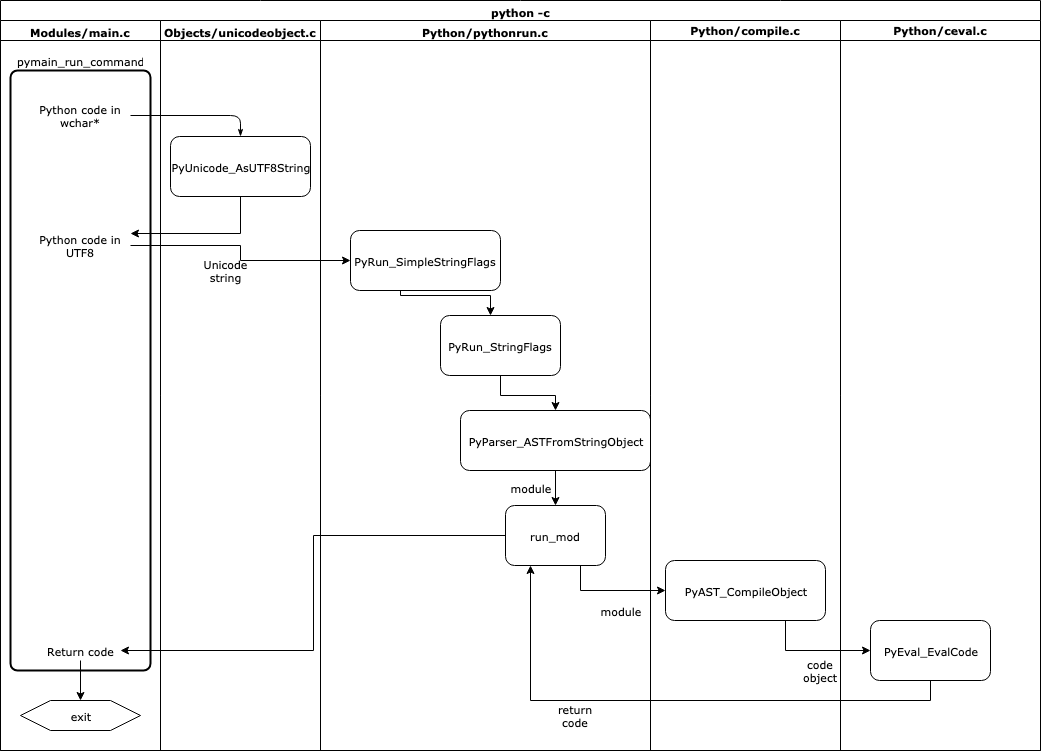
$ ./python.exe -c "print('hi')"hiHere is the full flowchart of how this happens:
![Flow chart of pymain_run_command]()
First, the pymain_run_command() function is executed inside Modules/main.c taking the command passed in -c as an argument in the C type wchar_t*. The wchar_t* type is often used as a low-level storage type for Unicode data across CPython as the size of the type can store UTF8 characters.
When converting the wchar_t* to a Python string, the Objects/unicodetype.c file has a helper function PyUnicode_FromWideChar() that returns a PyObject, of type str. The encoding to UTF8 is then done by PyUnicode_AsUTF8String() on the Python str object to convert it to a Python bytes object.
Once this is complete, pymain_run_command() will then pass the Python bytes object to PyRun_SimpleStringFlags() for execution, but first converting the bytes to a str type again:
staticintpymain_run_command(wchar_t*command,PyCompilerFlags*cf){PyObject*unicode,*bytes;intret;unicode=PyUnicode_FromWideChar(command,-1);if(unicode==NULL){gotoerror;}if(PySys_Audit("cpython.run_command","O",unicode)<0){returnpymain_exit_err_print();}bytes=PyUnicode_AsUTF8String(unicode);Py_DECREF(unicode);if(bytes==NULL){gotoerror;}ret=PyRun_SimpleStringFlags(PyBytes_AsString(bytes),cf);Py_DECREF(bytes);return(ret!=0);error:PySys_WriteStderr("Unable to decode the command from the command line:\n");returnpymain_exit_err_print();}The conversion of wchar_t* to Unicode, bytes, and then a string is roughly equivalent to the following:
unicode=str(command)bytes_=bytes(unicode.encode('utf8'))# call PyRun_SimpleStringFlags with bytes_The PyRun_SimpleStringFlags() function is part of Python/pythonrun.c. It’s purpose is to turn this simple command into a Python module and then send it on to be executed.
Since a Python module needs to have __main__ to be executed as a standalone module, it creates that automatically:
intPyRun_SimpleStringFlags(constchar*command,PyCompilerFlags*flags){PyObject*m,*d,*v;m=PyImport_AddModule("__main__");if(m==NULL)return-1;d=PyModule_GetDict(m);v=PyRun_StringFlags(command,Py_file_input,d,d,flags);if(v==NULL){PyErr_Print();return-1;}Py_DECREF(v);return0;}Once PyRun_SimpleStringFlags() has created a module and a dictionary, it calls PyRun_StringFlags(), which creates a fake filename and then calls the Python parser to create an AST from the string and return a module, mod:
PyObject*PyRun_StringFlags(constchar*str,intstart,PyObject*globals,PyObject*locals,PyCompilerFlags*flags){...mod=PyParser_ASTFromStringObject(str,filename,start,flags,arena);if(mod!=NULL)ret=run_mod(mod,filename,globals,locals,flags,arena);PyArena_Free(arena);returnret;You’ll dive into the AST and Parser code in the next section.
Another way to execute Python commands is by using the -m option with the name of a module.
A typical example is python -m unittest to run the unittest module in the standard library.
Being able to execute modules as scripts were initially proposed in PEP 338 and then the standard for explicit relative imports defined in PEP366.
The use of the -m flag implies that within the module package, you want to execute whatever is inside __main__. It also implies that you want to search sys.path for the named module.
This search mechanism is why you don’t need to remember where the unittest module is stored on your filesystem.
Inside Modules/main.c there is a function called when the command-line is run with the -m flag. The name of the module is passed as the modname argument.
CPython will then import a standard library module, runpy and execute it using PyObject_Call(). The import is done using the C API function PyImport_ImportModule(), found within the Python/import.c file:
staticintpymain_run_module(constwchar_t*modname,intset_argv0){PyObject*module,*runpy,*runmodule,*runargs,*result;runpy=PyImport_ImportModule("runpy");...runmodule=PyObject_GetAttrString(runpy,"_run_module_as_main");...module=PyUnicode_FromWideChar(modname,wcslen(modname));...runargs=Py_BuildValue("(Oi)",module,set_argv0);...result=PyObject_Call(runmodule,runargs,NULL);...if(result==NULL){returnpymain_exit_err_print();}Py_DECREF(result);return0;}In this function you’ll also see 2 other C API functions: PyObject_Call() and PyObject_GetAttrString(). Because PyImport_ImportModule() returns a PyObject*, the core object type, you need to call special functions to get attributes and to call it.
In Python, if you had an object and wanted to get an attribute, then you could call getattr(). In the C API, this call is PyObject_GetAttrString(), which is found in Objects/object.c. If you wanted to run a callable, you would give it parentheses, or you can run the __call__() property on any Python object. The __call__() method is implemented inside Objects/object.c:
hi="hi!"hi.upper()==hi.upper.__call__()# this is the same
The runpy module is written in pure Python and located in Lib/runpy.py.
Executing python -m <module> is equivalent to running python -m runpy <module>. The runpy module was created to abstract the process of locating and executing modules on an operating system.
runpy does a few things to run the target module:
- Calls
__import__() for the module name you provided - Sets
__name__ (the module name) to a namespace called __main__ - Executes the module within the
__main__ namespace
The runpy module also supports executing directories and zip files.
If the first argument to python was a filename, such as python test.py, then CPython will open a file handle, similar to using open() in Python and pass the handle to PyRun_SimpleFileExFlags() inside Python/pythonrun.c.
There are 3 paths this function can take:
- If the file path is a
.pyc file, it will call run_pyc_file(). - If the file path is a script file (
.py) it will run PyRun_FileExFlags(). - If the filepath is
stdin because the user ran command | python then treat stdin as a file handle and run PyRun_FileExFlags().
intPyRun_SimpleFileExFlags(FILE*fp,constchar*filename,intcloseit,PyCompilerFlags*flags){...m=PyImport_AddModule("__main__");...if(maybe_pyc_file(fp,filename,ext,closeit)){...v=run_pyc_file(pyc_fp,filename,d,d,flags);}else{/* When running from stdin, leave __main__.__loader__ alone */if(strcmp(filename,"<stdin>")!=0&&set_main_loader(d,filename,"SourceFileLoader")<0){fprintf(stderr,"python: failed to set __main__.__loader__\n");ret=-1;gotodone;}v=PyRun_FileExFlags(fp,filename,Py_file_input,d,d,closeit,flags);}...returnret;}For stdin and basic script files, CPython will pass the file handle to PyRun_FileExFlags() located in the pythonrun.c file.
The purpose of PyRun_FileExFlags() is similar to PyRun_SimpleStringFlags() used for the -c input. CPython will load the file handle into PyParser_ASTFromFileObject(). We’ll cover the Parser and AST modules in the next section.
Because this is a full script, it doesn’t need the PyImport_AddModule("__main__"); step used by -c:
PyObject*PyRun_FileExFlags(FILE*fp,constchar*filename_str,intstart,PyObject*globals,PyObject*locals,intcloseit,PyCompilerFlags*flags){...mod=PyParser_ASTFromFileObject(fp,filename,NULL,start,0,0,...ret=run_mod(mod,filename,globals,locals,flags,arena);}Identical to PyRun_SimpleStringFlags(), once PyRun_FileExFlags() has created a Python module from the file, it sent it to run_mod() to be executed.
run_mod() is found within Python/pythonrun.c, and sends the module to the AST to be compiled into a code object. Code objects are a format used to store the bytecode operations and the format kept in .pyc files:
staticPyObject*run_mod(mod_tymod,PyObject*filename,PyObject*globals,PyObject*locals,PyCompilerFlags*flags,PyArena*arena){PyCodeObject*co;PyObject*v;co=PyAST_CompileObject(mod,filename,flags,-1,arena);if(co==NULL)returnNULL;if(PySys_Audit("exec","O",co)<0){Py_DECREF(co);returnNULL;}v=run_eval_code_obj(co,globals,locals);Py_DECREF(co);returnv;}We will cover the CPython compiler and bytecodes in the next section. The call to run_eval_code_obj() is a simple wrapper function that calls PyEval_EvalCode() in the Python/eval.c file. The PyEval_EvalCode() function is the main evaluation loop for CPython, it iterates over each bytecode statement and executes it on your local machine.
In the PyRun_SimpleFileExFlags() there was a clause for the user providing a file path to a .pyc file. If the file path ended in .pyc then instead of loading the file as a plain text file and parsing it, it will assume that the .pyc file contains a code object written to disk.
The run_pyc_file() function inside Python/pythonrun.c then marshals the code object from the .pyc file by using the file handle. Marshaling is a technical term for copying the contents of a file into memory and converting them to a specific data structure. The code object data structure on the disk is the CPython compiler’s way to caching compiled code so that it doesn’t need to parse it every time the script is called:
staticPyObject*run_pyc_file(FILE*fp,constchar*filename,PyObject*globals,PyObject*locals,PyCompilerFlags*flags){PyCodeObject*co;PyObject*v;...v=PyMarshal_ReadLastObjectFromFile(fp);...if(v==NULL||!PyCode_Check(v)){Py_XDECREF(v);PyErr_SetString(PyExc_RuntimeError,"Bad code object in .pyc file");gotoerror;}fclose(fp);co=(PyCodeObject*)v;v=run_eval_code_obj(co,globals,locals);if(v&&flags)flags->cf_flags|=(co->co_flags&PyCF_MASK);Py_DECREF(co);returnv;}Once the code object has been marshaled to memory, it is sent to run_eval_code_obj(), which calls Python/ceval.c to execute the code.
Lexing and Parsing
In the exploration of reading and executing Python files, we dived as deep as the parser and AST modules, with function calls to PyParser_ASTFromFileObject().
Sticking within Python/pythonrun.c, the PyParser_ASTFromFileObject() function will take a file handle, compiler flags and a PyArena instance and convert the file object into a node object using PyParser_ParseFileObject().
With the node object, it will then convert that into a module using the AST function PyAST_FromNodeObject():
mod_tyPyParser_ASTFromFileObject(FILE*fp,PyObject*filename,constchar*enc,intstart,constchar*ps1,constchar*ps2,PyCompilerFlags*flags,int*errcode,PyArena*arena){...node*n=PyParser_ParseFileObject(fp,filename,enc,&_PyParser_Grammar,start,ps1,ps2,&err,&iflags);...if(n){flags->cf_flags|=iflags&PyCF_MASK;mod=PyAST_FromNodeObject(n,flags,filename,arena);PyNode_Free(n);...returnmod;}For PyParser_ParseFileObject() we switch to Parser/parsetok.c and the parser-tokenizer stage of the CPython interpreter. This function has two important tasks:
- Instantiate a tokenizer state
tok_state using PyTokenizer_FromFile() in Parser/tokenizer.c - Convert the tokens into a concrete parse tree (a list of
node) using parsetok() in Parser/parsetok.c
node*PyParser_ParseFileObject(FILE*fp,PyObject*filename,constchar*enc,grammar*g,intstart,constchar*ps1,constchar*ps2,perrdetail*err_ret,int*flags){structtok_state*tok;...if((tok=PyTokenizer_FromFile(fp,enc,ps1,ps2))==NULL){err_ret->error=E_NOMEM;returnNULL;}...returnparsetok(tok,g,start,err_ret,flags);}tok_state (defined in Parser/tokenizer.h) is the data structure to store all temporary data generated by the tokenizer. It is returned to the parser-tokenizer as the data structure is required by parsetok() to develop the concrete syntax tree.
Inside parsetok(), it will use the tok_state structure and make calls to tok_get() in a loop until the file is exhausted and no more tokens can be found.
tok_get(), defined in Parser/tokenizer.c behaves like an iterator. It will keep returning the next token in the parse tree.
tok_get() is one of the most complex functions in the whole CPython codebase. It has over 640 lines and includes decades of heritage with edge cases, new language features, and syntax.
One of the simpler examples would be the part that converts a newline break into a NEWLINE token:
staticinttok_get(structtok_state*tok,char**p_start,char**p_end){.../* Newline */if(c=='\n'){tok->atbol=1;if(blankline||tok->level>0){gotonextline;}*p_start=tok->start;*p_end=tok->cur-1;/* Leave '\n' out of the string */tok->cont_line=0;if(tok->async_def){/* We're somewhere inside an 'async def' function, and we've encountered a NEWLINE after its signature. */tok->async_def_nl=1;}returnNEWLINE;}...}In this case, NEWLINE is a token, with a value defined in Include/token.h. All tokens are constant int values, and the Include/token.h file was generated earlier when we ran make regen-grammar.
The node type returned by PyParser_ParseFileObject() is going to be essential for the next stage, converting a parse tree into an Abstract-Syntax-Tree (AST):
typedefstruct_node{shortn_type;char*n_str;intn_lineno;intn_col_offset;intn_nchildren;struct_node*n_child;intn_end_lineno;intn_end_col_offset;}node;Since the CST is a tree of syntax, token IDs, and symbols, it would be difficult for the compiler to make quick decisions based on the Python language.
That is why the next stage is to convert the CST into an AST, a much higher-level structure. This task is performed by the Python/ast.c module, which has both a C and Python API.
Before you jump into the AST, there is a way to access the output from the parser stage. CPython has a standard library module parser, which exposes the C functions with a Python API.
The module is documented as an implementation detail of CPython so that you won’t see it in other Python interpreters. Also the output from the functions is not that easy to read.
The output will be in the numeric form, using the token and symbol numbers generated by the make regen-grammar stage, stored in Include/token.h and Include/symbol.h:
>>>>>> frompprintimportpprint>>> importparser>>> st=parser.expr('a + 1')>>> pprint(parser.st2list(st))[258, [332, [306, [310, [311, [312, [313, [316, [317, [318, [319, [320, [321, [322, [323, [324, [325, [1, 'a']]]]]], [14, '+'], [321, [322, [323, [324, [325, [2, '1']]]]]]]]]]]]]]]]], [4, ''], [0, '']] To make it easier to understand, you can take all the numbers in the symbol and token modules, put them into a dictionary and recursively replace the values in the output of parser.st2list() with the names:
importsymbolimporttokenimportparserdeflex(expression):symbols={v:kfork,vinsymbol.__dict__.items()ifisinstance(v,int)}tokens={v:kfork,vintoken.__dict__.items()ifisinstance(v,int)}lexicon={**symbols,**tokens}st=parser.expr(expression)st_list=parser.st2list(st)defreplace(l:list):r=[]foriinl:ifisinstance(i,list):r.append(replace(i))else:ifiinlexicon:r.append(lexicon[i])else:r.append(i)returnrreturnreplace(st_list)You can run lex() with a simple expression, like a + 1 to see how this is represented as a parser-tree:
>>>>>> frompprintimportpprint>>> pprint(lex('a + 1'))['eval_input', ['testlist', ['test', ['or_test', ['and_test', ['not_test', ['comparison', ['expr', ['xor_expr', ['and_expr', ['shift_expr', ['arith_expr', ['term', ['factor', ['power', ['atom_expr', ['atom', ['NAME', 'a']]]]]], ['PLUS', '+'], ['term', ['factor', ['power', ['atom_expr', ['atom', ['NUMBER', '1']]]]]]]]]]]]]]]]], ['NEWLINE', ''], ['ENDMARKER', '']] In the output, you can see the symbols in lowercase, such as 'test' and the tokens in uppercase, such as 'NUMBER'.
Abstract Syntax Trees
The next stage in the CPython interpreter is to convert the CST generated by the parser into something more logical that can be executed. The structure is a higher-level representation of the code, called an Abstract Syntax Tree (AST).
ASTs are produced inline with the CPython interpreter process, but you can also generate them in both Python using the ast module in the Standard Library as well as through the C API.
Before diving into the C implementation of the AST, it would be useful to understand what an AST looks like for a simple piece of Python code.
To do this, here’s a simple app called instaviz for this tutorial. It displays the AST and bytecode instructions (which we’ll cover later) in a Web UI.
To install instaviz:
Then, open up a REPL by running python at the command line with no arguments:
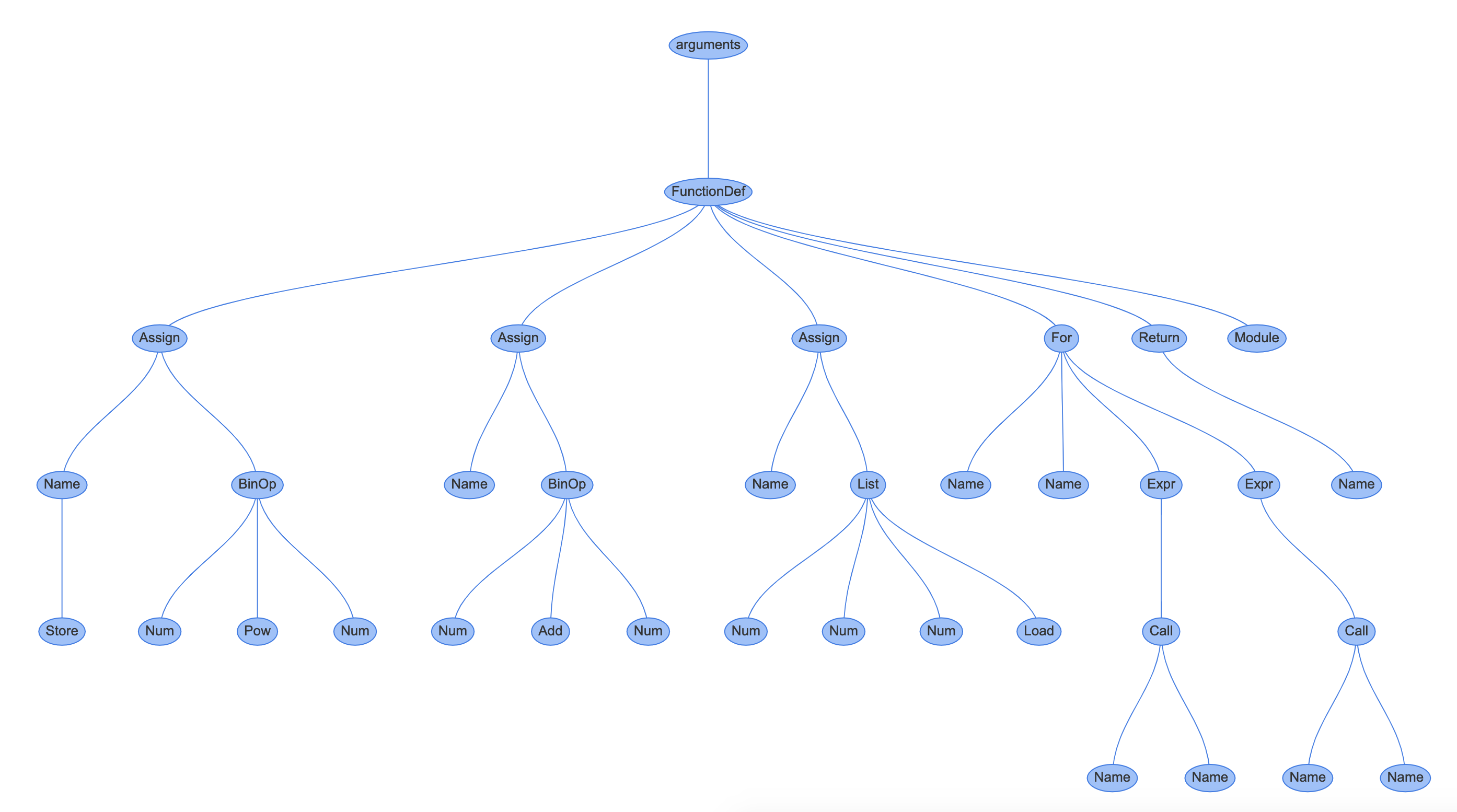
>>>>>> importinstaviz>>> defexample(): a = 1 b = a + 1 return b>>> instaviz.show(example)
You’ll see a notification on the command-line that a web server has started on port 8080. If you were using that port for something else, you can change it by calling instaviz.show(example, port=9090) or another port number.
In the web browser, you can see the detailed breakdown of your function:
![Instaviz screenshot]()
The bottom left graph is the function you declared in REPL, represented as an Abstract Syntax Tree. Each node in the tree is an AST type. They are found in the ast module, and all inherit from _ast.AST.
Some of the nodes have properties which link them to child nodes, unlike the CST, which has a generic child node property.
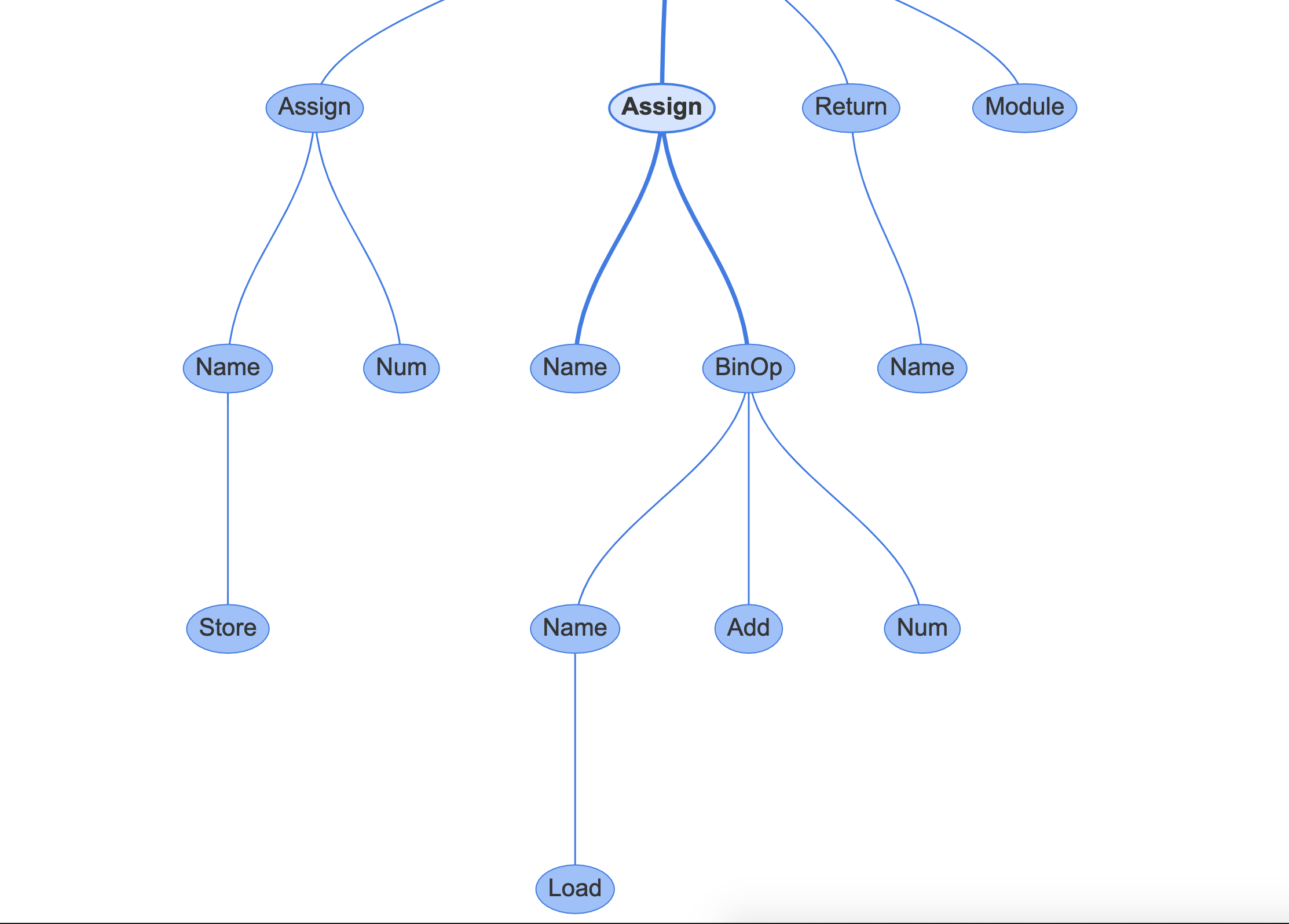
For example, if you click on the Assign node in the center, this links to the line b = a + 1:
![Instaviz screenshot 2]()
It has two properties:
targets is a list of names to assign. It is a list because you can assign to multiple variables with a single expression using unpackingvalue is the value to assign, which in this case is a BinOp statement, a + 1.
If you click on the BinOp statement, it shows the properties of relevance:
left: the node to the left of the operatorop: the operator, in this case, an Add node (+) for additionright: the node to the right of the operator
![Instaviz screenshot 3]()
Compiling an AST in C is not a straightforward task, so the Python/ast.c module is over 5000 lines of code.
There are a few entry points, forming part of the AST’s public API. In the last section on the lexer and parser, you stopped when you’d reached the call to PyAST_FromNodeObject(). By this stage, the Python interpreter process had created a CST in the format of node * tree.
Jumping then into PyAST_FromNodeObject() inside Python/ast.c, you can see it receives the node * tree, the filename, compiler flags, and the PyArena.
The return type from this function is mod_ty, defined in Include/Python-ast.h. mod_ty is a container structure for one of the 5 module types in Python:
ModuleInteractiveExpressionFunctionTypeSuite
In Include/Python-ast.h you can see that an Expression type requires a field body, which is an expr_ty type. The expr_ty type is also defined in Include/Python-ast.h:
enum_mod_kind{Module_kind=1,Interactive_kind=2,Expression_kind=3,FunctionType_kind=4,Suite_kind=5};struct_mod{enum_mod_kindkind;union{struct{asdl_seq*body;asdl_seq*type_ignores;}Module;struct{asdl_seq*body;}Interactive;struct{expr_tybody;}Expression;struct{asdl_seq*argtypes;expr_tyreturns;}FunctionType;struct{asdl_seq*body;}Suite;}v;};The AST types are all listed in Parser/Python.asdl. You will see the module types, statement types, expression types, operators, and comprehensions all listed. The names of the types in this document relate to the classes generated by the AST and the same classes named in the ast standard module library.
The parameters and names in Include/Python-ast.h correlate directly to those specified in Parser/Python.asdl:
-- ASDL's 5 builtin types are:
-- identifier, int, string, object, constant

module Python
{
    mod = Module(stmt* body, type_ignore *type_ignores)
        | Interactive(stmt* body)
        | Expression(expr body)
        | FunctionType(expr* argtypes, expr returns)
The C header file and structures are there so that the Python/ast.c program can quickly generate the structures with pointers to the relevant data.
Looking at PyAST_FromNodeObject() you can see that it is essentially a switch statement around the result from TYPE(n). TYPE() is one of the core functions used by the AST to determine what type a node in the concrete syntax tree is. In the case of PyAST_FromNodeObject() it’s just looking at the first node, so it can only be one of the module types defined as Module, Interactive, Expression, FunctionType.
The result of TYPE() will be either a symbol or token type, which we’re very familiar with by this stage.
For file_input, the results should be a Module. Modules are a series of statements, of which there are a few types. The logic to traverse the children of n and create statement nodes is within ast_for_stmt(). This function is called either once, if there is only 1 statement in the module, or in a loop if there are many. The resulting Module is then returned with the PyArena.
For eval_input, the result should be an Expression. The result from CHILD(n ,0), which is the first child of n is passed to ast_for_testlist() which returns an expr_ty type. This expr_ty is sent to Expression() with the PyArena to create an expression node, and then passed back as a result:
mod_tyPyAST_FromNodeObject(constnode*n,PyCompilerFlags*flags,PyObject*filename,PyArena*arena){...switch(TYPE(n)){casefile_input:stmts=_Py_asdl_seq_new(num_stmts(n),arena);if(!stmts)gotoout;for(i=0;i<NCH(n)-1;i++){ch=CHILD(n,i);if(TYPE(ch)==NEWLINE)continue;REQ(ch,stmt);num=num_stmts(ch);if(num==1){s=ast_for_stmt(&c,ch);if(!s)gotoout;asdl_seq_SET(stmts,k++,s);}else{ch=CHILD(ch,0);REQ(ch,simple_stmt);for(j=0;j<num;j++){s=ast_for_stmt(&c,CHILD(ch,j*2));if(!s)gotoout;asdl_seq_SET(stmts,k++,s);}}}/* Type ignores are stored under the ENDMARKER in file_input. */...res=Module(stmts,type_ignores,arena);break;caseeval_input:{expr_tytestlist_ast;/* XXX Why not comp_for here? */testlist_ast=ast_for_testlist(&c,CHILD(n,0));if(!testlist_ast)gotoout;res=Expression(testlist_ast,arena);break;}casesingle_input:...break;casefunc_type_input:......returnres;}Inside the ast_for_stmt() function, there is another switch statement for each possible statement type (simple_stmt, compound_stmt, and so on) and the code to determine the arguments to the node class.
One of the simpler functions is for the power expression, i.e., 2**4 is 2 to the power of 4. This function starts by getting the ast_for_atom_expr(), which is the number 2 in our example, then if that has one child, it returns the atomic expression. If it has more than one child, it will get the right-hand (the number 4) and return a BinOp (binary operation) with the operator as Pow (power), the left hand of e (2), and the right hand of f (4):
staticexpr_tyast_for_power(structcompiling*c,constnode*n){/* power: atom trailer* ('**' factor)* */expr_tye;REQ(n,power);e=ast_for_atom_expr(c,CHILD(n,0));if(!e)returnNULL;if(NCH(n)==1)returne;if(TYPE(CHILD(n,NCH(n)-1))==factor){expr_tyf=ast_for_expr(c,CHILD(n,NCH(n)-1));if(!f)returnNULL;e=BinOp(e,Pow,f,LINENO(n),n->n_col_offset,n->n_end_lineno,n->n_end_col_offset,c->c_arena);}returne;}You can see the result of this if you send a short function to the instaviz module:
>>>>>> deffoo(): 2**4>>> importinstaviz>>> instaviz.show(foo)
![Instaviz screenshot 4]()
In the UI you can also see the corresponding properties:
![Instaviz screenshot 5]()
In summary, each statement type and expression has a corresponding ast_for_*() function to create it. The arguments are defined in Parser/Python.asdl and exposed via the ast module in the standard library. If an expression or statement has children, then it will call the corresponding ast_for_* child function in a depth-first traversal.
Conclusion
CPython’s versatility and low-level execution API make it the ideal candidate for an embedded scripting engine. You will see CPython used in many UI applications, such as Game Design, 3D graphics and system automation.
The interpreter process is flexible and efficient, and now you have an understanding of how it works you’re ready to understand the compiler.
Part 3: The CPython Compiler and Execution Loop
In Part 2, you saw how the CPython interpreter takes an input, such as a file or string, and converts it into a logical Abstract Syntax Tree. We’re still not at the stage where this code can be executed. Next, we have to go deeper to convert the Abstract Syntax Tree into a set of sequential commands that the CPU can understand.
Compiling
Now the interpreter has an AST with the properties required for each of the operations, functions, classes, and namespaces. It is the job of the compiler to turn the AST into something the CPU can understand.
This compilation task is split into 2 parts:
- Traverse the tree and create a control-flow-graph, which represents the logical sequence for execution
- Convert the nodes in the CFG to smaller, executable statements, known as byte-code
Earlier, we were looking at how files are executed, and the PyRun_FileExFlags() function in Python/pythonrun.c. Inside this function, we converted the FILE handle into a mod, of type mod_ty. This task was completed by PyParser_ASTFromFileObject(), which in turns calls the tokenizer, parser-tokenizer and then the AST:
PyObject*PyRun_FileExFlags(FILE*fp,constchar*filename_str,intstart,PyObject*globals,PyObject*locals,intcloseit,PyCompilerFlags*flags){...mod=PyParser_ASTFromFileObject(fp,filename,NULL,start,0,0,...ret=run_mod(mod,filename,globals,locals,flags,arena);}The resulting module from the call to is sent to run_mod() still in Python/pythonrun.c. This is a small function that gets a PyCodeObject from PyAST_CompileObject() and sends it on to run_eval_code_obj(). You will tackle run_eval_code_obj() in the next section:
staticPyObject*run_mod(mod_tymod,PyObject*filename,PyObject*globals,PyObject*locals,PyCompilerFlags*flags,PyArena*arena){PyCodeObject*co;PyObject*v;co=PyAST_CompileObject(mod,filename,flags,-1,arena);if(co==NULL)returnNULL;if(PySys_Audit("exec","O",co)<0){Py_DECREF(co);returnNULL;}v=run_eval_code_obj(co,globals,locals);Py_DECREF(co);returnv;}The PyAST_CompileObject() function is the main entry point to the CPython compiler. It takes a Python module as its primary argument, along with the name of the file, the globals, locals, and the PyArena all created earlier in the interpreter process.
We’re starting to get into the guts of the CPython compiler now, with decades of development and Computer Science theory behind it. Don’t be put off by the language. Once we break down the compiler into logical steps, it’ll make sense.
Before the compiler starts, a global compiler state is created. This type, compiler is defined in Python/compile.c and contains properties used by the compiler to remember the compiler flags, the stack, and the PyArena:
structcompiler{PyObject*c_filename;structsymtable*c_st;PyFutureFeatures*c_future;/* pointer to module's __future__ */PyCompilerFlags*c_flags;intc_optimize;/* optimization level */intc_interactive;/* true if in interactive mode */intc_nestlevel;PyObject*c_const_cache;/* Python dict holding all constants, including names tuple */structcompiler_unit*u;/* compiler state for current block */PyObject*c_stack;/* Python list holding compiler_unit ptrs */PyArena*c_arena;/* pointer to memory allocation arena */};Inside PyAST_CompileObject(), there are 11 main steps happening:
- Create an empty
__doc__ property to the module if it doesn’t exist. - Create an empty
__annotations__ property to the module if it doesn’t exist. - Set the filename of the global compiler state to the filename argument.
- Set the memory allocation arena for the compiler to the one used by the interpreter.
- Copy any
__future__ flags in the module to the future flags in the compiler. - Merge runtime flags provided by the command-line or environment variables.
- Enable any
__future__ features in the compiler. - Set the optimization level to the provided argument, or default.
- Build a symbol table from the module object.
- Run the compiler with the compiler state and return the code object.
- Free any allocated memory by the compiler.
PyCodeObject*PyAST_CompileObject(mod_tymod,PyObject*filename,PyCompilerFlags*flags,intoptimize,PyArena*arena){structcompilerc;PyCodeObject*co=NULL;PyCompilerFlagslocal_flags;intmerged;if(!__doc__){// 1.__doc__=PyUnicode_InternFromString("__doc__");if(!__doc__)returnNULL;}if(!__annotations__){__annotations__=PyUnicode_InternFromString("__annotations__");// 2.if(!__annotations__)returnNULL;}if(!compiler_init(&c))returnNULL;Py_INCREF(filename);c.c_filename=filename;// 3.c.c_arena=arena;// 4.c.c_future=PyFuture_FromASTObject(mod,filename);// 5.if(c.c_future==NULL)gotofinally;if(!flags){local_flags.cf_flags=0;local_flags.cf_feature_version=PY_MINOR_VERSION;flags=&local_flags;}merged=c.c_future->ff_features|flags->cf_flags;// 6.c.c_future->ff_features=merged;// 7.flags->cf_flags=merged;c.c_flags=flags;c.c_optimize=(optimize==-1)?Py_OptimizeFlag:optimize;// 8.c.c_nestlevel=0;if(!_PyAST_Optimize(mod,arena,c.c_optimize)){gotofinally;}c.c_st=PySymtable_BuildObject(mod,filename,c.c_future);// 9.if(c.c_st==NULL){if(!PyErr_Occurred())PyErr_SetString(PyExc_SystemError,"no symtable");gotofinally;}co=compiler_mod(&c,mod);// 10.finally:compiler_free(&c);// 11.assert(co||PyErr_Occurred());returnco;}Future Flags and Compiler Flags
Before the compiler runs, there are two types of flags to toggle the features inside the compiler. These come from two places:
- The interpreter state, which may have been command-line options, set in
pyconfig.h or via environment variables - The use of
__future__ statements inside the actual source code of the module
To distinguish the two types of flags, think that the __future__ flags are required because of the syntax or features in that specific module. For example, Python 3.7 introduced delayed evaluation of type hints through the annotations future flag:
from__future__importannotations
The code after this statement might use unresolved type hints, so the __future__ statement is required. Otherwise, the module wouldn’t import. It would be unmaintainable to manually request that the person importing the module enable this specific compiler flag.
The other compiler flags are specific to the environment, so they might change the way the code executes or the way the compiler runs, but they shouldn’t link to the source in the same way that __future__ statements do.
One example of a compiler flag would be the -O flag for optimizing the use of assert statements. This flag disables any assert statements, which may have been put in the code for debugging purposes.
It can also be enabled with the PYTHONOPTIMIZE=1 environment variable setting.
Symbol Tables
In PyAST_CompileObject() there was a reference to a symtable and a call to PySymtable_BuildObject() with the module to be executed.
The purpose of the symbol table is to provide a list of namespaces, globals, and locals for the compiler to use for referencing and resolving scopes.
The symtable structure in Include/symtable.h is well documented, so it’s clear what each of the fields is for. There should be one symtable instance for the compiler, so namespacing becomes essential.
If you create a function called resolve_names() in one module and declare another function with the same name in another module, you want to be sure which one is called. The symtable serves this purpose, as well as ensuring that variables declared within a narrow scope don’t automatically become globals (after all, this isn’t JavaScript):
structsymtable{PyObject*st_filename;/* name of file being compiled, decoded from the filesystem encoding */struct_symtable_entry*st_cur;/* current symbol table entry */struct_symtable_entry*st_top;/* symbol table entry for module */PyObject*st_blocks;/* dict: map AST node addresses * to symbol table entries */PyObject*st_stack;/* list: stack of namespace info */PyObject*st_global;/* borrowed ref to st_top->ste_symbols */intst_nblocks;/* number of blocks used. kept for consistency with the corresponding compiler structure */PyObject*st_private;/* name of current class or NULL */PyFutureFeatures*st_future;/* module's future features that affect the symbol table */intrecursion_depth;/* current recursion depth */intrecursion_limit;/* recursion limit */};Some of the symbol table API is exposed via the symtable module in the standard library. You can provide an expression or a module an receive a symtable.SymbolTable instance.
You can provide a string with a Python expression and the compile_type of "eval", or a module, function or class, and the compile_mode of "exec" to get a symbol table.
Looping over the elements in the table we can see some of the public and private fields and their types:
>>>>>> importsymtable>>> s=symtable.symtable('b + 1',filename='test.py',compile_type='eval')>>> [symbol.__dict__forsymbolins.get_symbols()][{'_Symbol__name': 'b', '_Symbol__flags': 6160, '_Symbol__scope': 3, '_Symbol__namespaces': ()}] The C code behind this is all within Python/symtable.c and the primary interface is the PySymtable_BuildObject() function.
Similar to the top-level AST function we covered earlier, the PySymtable_BuildObject() function switches between the mod_ty possible types (Module, Expression, Interactive, Suite, FunctionType), and visits each of the statements inside them.
Remember, mod_ty is an AST instance, so the will now recursively explore the nodes and branches of the tree and add entries to the symtable:
structsymtable*PySymtable_BuildObject(mod_tymod,PyObject*filename,PyFutureFeatures*future){structsymtable*st=symtable_new();asdl_seq*seq;inti;PyThreadState*tstate;intrecursion_limit=Py_GetRecursionLimit();...st->st_top=st->st_cur;switch(mod->kind){caseModule_kind:seq=mod->v.Module.body;for(i=0;i<asdl_seq_LEN(seq);i++)if(!symtable_visit_stmt(st,(stmt_ty)asdl_seq_GET(seq,i)))gotoerror;break;caseExpression_kind:...caseInteractive_kind:...caseSuite_kind:...caseFunctionType_kind:...}...}So for a module, PySymtable_BuildObject() will loop through each statement in the module and call symtable_visit_stmt(). The symtable_visit_stmt() is a huge switch statement with a case for each statement type (defined in Parser/Python.asdl).
For each statement type, there is specific logic to that statement type. For example, a function definition has particular logic for:
- If the recursion depth is beyond the limit, raise a recursion depth error
- The name of the function to be added as a local variable
- The default values for sequential arguments to be resolved
- The default values for keyword arguments to be resolved
- Any annotations for the arguments or the return type are resolved
- Any function decorators are resolved
- The code block with the contents of the function is visited in
symtable_enter_block() - The arguments are visited
- The body of the function is visited
Note: If you’ve ever wondered why Python’s default arguments are mutable, the reason is in this function. You can see they are a pointer to the variable in the symtable. No extra work is done to copy any values to an immutable type.
staticintsymtable_visit_stmt(structsymtable*st,stmt_tys){if(++st->recursion_depth>st->recursion_limit){// 1.PyErr_SetString(PyExc_RecursionError,"maximum recursion depth exceeded during compilation");VISIT_QUIT(st,0);}switch(s->kind){caseFunctionDef_kind:if(!symtable_add_def(st,s->v.FunctionDef.name,DEF_LOCAL))// 2.VISIT_QUIT(st,0);if(s->v.FunctionDef.args->defaults)// 3.VISIT_SEQ(st,expr,s->v.FunctionDef.args->defaults);if(s->v.FunctionDef.args->kw_defaults)// 4.VISIT_SEQ_WITH_NULL(st,expr,s->v.FunctionDef.args->kw_defaults);if(!symtable_visit_annotations(st,s,s->v.FunctionDef.args,// 5.s->v.FunctionDef.returns))VISIT_QUIT(st,0);if(s->v.FunctionDef.decorator_list)// 6.VISIT_SEQ(st,expr,s->v.FunctionDef.decorator_list);if(!symtable_enter_block(st,s->v.FunctionDef.name,// 7.FunctionBlock,(void*)s,s->lineno,s->col_offset))VISIT_QUIT(st,0);VISIT(st,arguments,s->v.FunctionDef.args);// 8.VISIT_SEQ(st,stmt,s->v.FunctionDef.body);// 9.if(!symtable_exit_block(st,s))VISIT_QUIT(st,0);break;caseClassDef_kind:{...}caseReturn_kind:...caseDelete_kind:...caseAssign_kind:...caseAnnAssign_kind:...Once the resulting symtable has been created, it is sent back to be used for the compiler.
Core Compilation Process
Now that the PyAST_CompileObject() has a compiler state, a symtable, and a module in the form of the AST, the actual compilation can begin.
The purpose of the core compiler is to:
- Convert the state, symtable, and AST into a Control-Flow-Graph (CFG)
- Protect the execution stage from runtime exceptions by catching any logic and code errors and raising them here
You can call the CPython compiler in Python code by calling the built-in function compile(). It returns a code object instance:
>>>>>> compile('b+1','test.py',mode='eval')<code object <module> at 0x10f222780, file "test.py", line 1> The same as with the symtable() function, a simple expression should have a mode of 'eval' and a module, function, or class should have a mode of 'exec'.
The compiled code can be found in the co_code property of the code object:
>>>>>> co.co_codeb'e\x00d\x00\x17\x00S\x00'
There is also a dis module in the standard library, which disassembles the bytecode instructions and can print them on the screen or give you a list of Instruction instances.
If you import dis and give the dis() function the code object’s co_code property it disassembles it and prints the instructions on the REPL:
>>> import dis
>>> dis.dis(co.co_code)
          0 LOAD_NAME                0 (0)
          2 LOAD_CONST               0 (0)
          4 BINARY_ADD
          6 RETURN_VALUE
LOAD_NAME, LOAD_CONST, BINARY_ADD, and RETURN_VALUE are all bytecode instructions. They’re called bytecode because, in binary form, they were a byte long. However, since Python 3.6 the storage format was changed to a word, so now they’re technically wordcode, not bytecode.
The full list of bytecode instructions is available for each version of Python, and it does change between versions. For example, in Python 3.7, some new bytecode instructions were introduced to speed up execution of specific method calls.
In an earlier section, we explored the instaviz package. This included a visualization of the code object type by running the compiler. It also displays the Bytecode operations inside the code objects.
Execute instaviz again to see the code object and bytecode for a function defined on the REPL:
>>>>>> importinstaviz>>> defexample(): a = 1 b = a + 1 return b>>> instaviz.show(example)
If we now jump into compiler_mod(), a function used to switch to different compiler functions depending on the module type. We’ll assume that mod is a Module. The module is compiled into the compiler state and then assemble() is run to create a PyCodeObject.
The new code object is returned back to PyAST_CompileObject() and sent on for execution:
staticPyCodeObject*compiler_mod(structcompiler*c,mod_tymod){PyCodeObject*co;intaddNone=1;staticPyObject*module;...switch(mod->kind){caseModule_kind:if(!compiler_body(c,mod->v.Module.body)){compiler_exit_scope(c);return0;}break;caseInteractive_kind:...caseExpression_kind:...caseSuite_kind:......co=assemble(c,addNone);compiler_exit_scope(c);returnco;}The compiler_body() function has some optimization flags and then loops over each statement in the module and visits it, similar to how the symtable functions worked:
staticintcompiler_body(structcompiler*c,asdl_seq*stmts){inti=0;stmt_tyst;PyObject*docstring;...for(;i<asdl_seq_LEN(stmts);i++)VISIT(c,stmt,(stmt_ty)asdl_seq_GET(stmts,i));return1;}The statement type is determined through a call to the asdl_seq_GET() function, which looks at the AST node’s type.
Through some smart macros, VISIT calls a function in Python/compile.c for each statement type:
#define VISIT(C, TYPE, V) {\ if (!compiler_visit_ ## TYPE((C), (V))) \ return 0; \}For a stmt (the category for a statement) the compiler will then drop into compiler_visit_stmt() and switch through all of the potential statement types found in Parser/Python.asdl:
staticintcompiler_visit_stmt(structcompiler*c,stmt_tys){Py_ssize_ti,n;/* Always assign a lineno to the next instruction for a stmt. */c->u->u_lineno=s->lineno;c->u->u_col_offset=s->col_offset;c->u->u_lineno_set=0;switch(s->kind){caseFunctionDef_kind:returncompiler_function(c,s,0);caseClassDef_kind:returncompiler_class(c,s);...caseFor_kind:returncompiler_for(c,s);...}return1;}As an example, let’s focus on the For statement, in Python is the:
foriiniterable:# blockelse:# optional if iterable is False# block
If the statement is a For type, it calls compiler_for(). There is an equivalent compiler_*() function for all of the statement and expression types. The more straightforward types create the bytecode instructions inline, some of the more complex statement types call other functions.
Many of the statements can have sub-statements. A for loop has a body, but you can also have complex expressions in the assignment and the iterator.
The compiler’s compiler_ statements sends blocks to the compiler state. These blocks contain instructions, the instruction data structure in Python/compile.c has the opcode, any arguments, and the target block (if this is a jump instruction), it also contains the line number.
For jump statements, they can either be absolute or relative jump statements. Jump statements are used to “jump” from one operation to another. Absolute jump statements specify the exact operation number in the compiled code object, whereas relative jump statements specify the jump target relative to another operation:
structinstr{unsignedi_jabs:1;unsignedi_jrel:1;unsignedchari_opcode;inti_oparg;structbasicblock_*i_target;/* target block (if jump instruction) */inti_lineno;};So a frame block (of type basicblock), contains the following fields:
- A
b_list pointer, the link to a list of blocks for the compiler state - A list of instructions
b_instr, with both the allocated list size b_ialloc, and the number used b_iused - The next block after this one
b_next - Whether the block has been “seen” by the assembler when traversing depth-first
- If this block has a
RETURN_VALUE opcode (b_return) - The depth of the stack when this block was entered (
b_startdepth) - The instruction offset for the assembler
typedefstructbasicblock_{/* Each basicblock in a compilation unit is linked via b_list in the reverse order that the block are allocated. b_list points to the next block, not to be confused with b_next, which is next by control flow. */structbasicblock_*b_list;/* number of instructions used */intb_iused;/* length of instruction array (b_instr) */intb_ialloc;/* pointer to an array of instructions, initially NULL */structinstr*b_instr;/* If b_next is non-NULL, it is a pointer to the next block reached by normal control flow. */structbasicblock_*b_next;/* b_seen is used to perform a DFS of basicblocks. */unsignedb_seen:1;/* b_return is true if a RETURN_VALUE opcode is inserted. */unsignedb_return:1;/* depth of stack upon entry of block, computed by stackdepth() */intb_startdepth;/* instruction offset for block, computed by assemble_jump_offsets() */intb_offset;}basicblock;The For statement is somewhere in the middle in terms of complexity. There are 15 steps in the compilation of a For statement with the for <target> in <iterator>: syntax:
- Create a new code block called
start, this allocates memory and creates a basicblock pointer - Create a new code block called
cleanup - Create a new code block called
end - Push a frame block of type
FOR_LOOP to the stack with start as the entry block and end as the exit block - Visit the iterator expression, which adds any operations for the iterator
- Add the
GET_ITER operation to the compiler state - Switch to the
start block - Call
ADDOP_JREL which calls compiler_addop_j() to add the FOR_ITER operation with an argument of the cleanup block - Visit the
target and add any special code, like tuple unpacking, to the start block - Visit each statement in the body of the for loop
- Call
ADDOP_JABS which calls compiler_addop_j() to add the JUMP_ABSOLUTE operation which indicates after the body is executed, jumps back to the start of the loop - Move to the
cleanup block - Pop the
FOR_LOOP frame block off the stack - Visit the statements inside the
else section of the for loop - Use the
end block
Referring back to the basicblock structure. You can see how in the compilation of the for statement, the various blocks are created and pushed into the compiler’s frame block and stack:
staticintcompiler_for(structcompiler*c,stmt_tys){basicblock*start,*cleanup,*end;start=compiler_new_block(c);// 1.cleanup=compiler_new_block(c);// 2.end=compiler_new_block(c);// 3.if(start==NULL||end==NULL||cleanup==NULL)return0;if(!compiler_push_fblock(c,FOR_LOOP,start,end))// 4.return0;VISIT(c,expr,s->v.For.iter);// 5.ADDOP(c,GET_ITER);// 6.compiler_use_next_block(c,start);// 7.ADDOP_JREL(c,FOR_ITER,cleanup);// 8.VISIT(c,expr,s->v.For.target);// 9.VISIT_SEQ(c,stmt,s->v.For.body);// 10.ADDOP_JABS(c,JUMP_ABSOLUTE,start);// 11.compiler_use_next_block(c,cleanup);// 12.compiler_pop_fblock(c,FOR_LOOP,start);// 13.VISIT_SEQ(c,stmt,s->v.For.orelse);// 14.compiler_use_next_block(c,end);// 15.return1;}Depending on the type of operation, there are different arguments required. For example, we used ADDOP_JABS and ADDOP_JREL here, which refer to “ADDOperation with Jump to a RELative position” and “ADDOperation with Jump to an ABSolute position”. This is referring to the APPOP_JREL and ADDOP_JABS macros which call compiler_addop_j(struct compiler *c, int opcode, basicblock *b, int absolute) and set the absolute argument to 0 and 1 respectively.
There are some other macros, like ADDOP_I calls compiler_addop_i() which add an operation with an integer argument, or ADDOP_O calls compiler_addop_o() which adds an operation with a PyObject argument.
Once these stages have completed, the compiler has a list of frame blocks, each containing a list of instructions and a pointer to the next block.
Assembly
With the compiler state, the assembler performs a “depth-first-search” of the blocks and merge the instructions into a single bytecode sequence. The assembler state is declared in Python/compile.c:
structassembler{PyObject*a_bytecode;/* string containing bytecode */inta_offset;/* offset into bytecode */inta_nblocks;/* number of reachable blocks */basicblock**a_postorder;/* list of blocks in dfs postorder */PyObject*a_lnotab;/* string containing lnotab */inta_lnotab_off;/* offset into lnotab */inta_lineno;/* last lineno of emitted instruction */inta_lineno_off;/* bytecode offset of last lineno */};The assemble() function has a few tasks:
- Calculate the number of blocks for memory allocation
- Ensure that every block that falls off the end returns
None, this is why every function returns None, whether or not a return statement exists - Resolve any jump statements offsets that were marked as relative
- Call
dfs() to perform a depth-first-search of the blocks - Emit all the instructions to the compiler
- Call
makecode() with the compiler state to generate the PyCodeObject
staticPyCodeObject*assemble(structcompiler*c,intaddNone){basicblock*b,*entryblock;structassemblera;inti,j,nblocks;PyCodeObject*co=NULL;/* Make sure every block that falls off the end returns None. XXX NEXT_BLOCK() isn't quite right, because if the last block ends with a jump or return b_next shouldn't set. */if(!c->u->u_curblock->b_return){NEXT_BLOCK(c);if(addNone)ADDOP_LOAD_CONST(c,Py_None);ADDOP(c,RETURN_VALUE);}...dfs(c,entryblock,&a,nblocks);/* Can't modify the bytecode after computing jump offsets. */assemble_jump_offsets(&a,c);/* Emit code in reverse postorder from dfs. */for(i=a.a_nblocks-1;i>=0;i--){b=a.a_postorder[i];for(j=0;j<b->b_iused;j++)if(!assemble_emit(&a,&b->b_instr[j]))gotoerror;}...co=makecode(c,&a);error:assemble_free(&a);returnco;}The depth-first-search is performed by the dfs() function in Python/compile.c, which follows the the b_next pointers in each of the blocks, marks them as seen by toggling b_seen and then adds them to the assemblers **a_postorder list in reverse order.
The function loops back over the assembler’s post-order list and for each block, if it has a jump operation, recursively call dfs() for that jump:
staticvoiddfs(structcompiler*c,basicblock*b,structassembler*a,intend){inti,j;/* Get rid of recursion for normal control flow. Since the number of blocks is limited, unused space in a_postorder (from a_nblocks to end) can be used as a stack for still not ordered blocks. */for(j=end;b&&!b->b_seen;b=b->b_next){b->b_seen=1;assert(a->a_nblocks<j);a->a_postorder[--j]=b;}while(j<end){b=a->a_postorder[j++];for(i=0;i<b->b_iused;i++){structinstr*instr=&b->b_instr[i];if(instr->i_jrel||instr->i_jabs)dfs(c,instr->i_target,a,j);}assert(a->a_nblocks<j);a->a_postorder[a->a_nblocks++]=b;}}Creating a Code Object
The task of makecode() is to go through the compiler state, some of the assembler’s properties and to put these into a PyCodeObject by calling PyCode_New():
![PyCodeObject structure]()
The variable names, constants are put as properties to the code object:
staticPyCodeObject*makecode(structcompiler*c,structassembler*a){...consts=consts_dict_keys_inorder(c->u->u_consts);names=dict_keys_inorder(c->u->u_names,0);varnames=dict_keys_inorder(c->u->u_varnames,0);...cellvars=dict_keys_inorder(c->u->u_cellvars,0);...freevars=dict_keys_inorder(c->u->u_freevars,PyTuple_GET_SIZE(cellvars));...flags=compute_code_flags(c);if(flags<0)gotoerror;bytecode=PyCode_Optimize(a->a_bytecode,consts,names,a->a_lnotab);...co=PyCode_New(argcount,kwonlyargcount,nlocals_int,maxdepth,flags,bytecode,consts,names,varnames,freevars,cellvars,c->c_filename,c->u->u_name,c->u->u_firstlineno,a->a_lnotab);...returnco;}You may also notice that the bytecode is sent to PyCode_Optimize() before it is sent to PyCode_New(). This function is part of the bytecode optimization process in Python/peephole.c.
The peephole optimizer goes through the bytecode instructions and in certain scenarios, replace them with other instructions. For example, there is an optimizer called “constant unfolding”, so if you put the following statement into your script:
It optimizes that to:
Because 1 and 5 are constant values, so the result should always be the same.
Conclusion
We can pull together all of these stages with the instaviz module:
importinstavizdeffoo():a=2**4b=1+5c=[1,4,6]foriinc:print(i)else:print(a)returncinstaviz.show(foo)
Will produce an AST graph:
![Instaviz screenshot 6]()
With bytecode instructions in sequence:
![Instaviz screenshot 7]()
Also, the code object with the variable names, constants, and binary co_code:
![Instaviz screenshot 8]()
Execution
In Python/pythonrun.c we broke out just before the call to run_eval_code_obj().
This call takes a code object, either fetched from the marshaled .pyc file, or compiled through the AST and compiler stages.
run_eval_code_obj() will pass the globals, locals, PyArena, and compiled PyCodeObject to PyEval_EvalCode() in Python/ceval.c.
This stage forms the execution component of CPython. Each of the bytecode operations is taken and executed using a “Stack Frame” based system.
What is a Stack Frame?
Stack Frames are a data type used by many runtimes, not just Python, that allows functions to be called and variables to be returned between functions. Stack Frames also contain arguments, local variables, and other state information.
Typically, a Stack Frame exists for every function call, and they are stacked in sequence. You can see CPython’s frame stack anytime an exception is unhandled and the stack is printed on the screen.
PyEval_EvalCode() is the public API for evaluating a code object. The logic for evaluation is split between _PyEval_EvalCodeWithName() and _PyEval_EvalFrameDefault(), which are both in ceval.c.
The public API PyEval_EvalCode() will construct an execution frame from the top of the stack by calling _PyEval_EvalCodeWithName().
The construction of the first execution frame has many steps:
- Keyword and positional arguments are resolved.
- The use of
*args and **kwargs in function definitions are resolved. - Arguments are added as local variables to the scope.
- Co-routines and Generators are created, including the Asynchronous Generators.
The frame object looks like this:
![PyFrameObject structure]()
Let’s step through those sequences.
1. Constructing Thread State
Before a frame can be executed, it needs to be referenced from a thread. CPython can have many threads running at any one time within a single interpreter. An Interpreter state includes a list of those threads as a linked list. The thread structure is called PyThreadState, and there are many references throughout ceval.c.
Here is the structure of the thread state object:
![PyThreadState structure]()
2. Constructing Frames
The input to PyEval_EvalCode() and therefore _PyEval_EvalCodeWithName() has arguments for:
_co: a PyCodeObjectglobals: a PyDict with variable names as keys and their valueslocals: a PyDict with variable names as keys and their values
The other arguments are optional, and not used for the basic API:
args: a PyTuple with positional argument values in order, and argcount for the number of valueskwnames: a list of keyword argument nameskwargs: a list of keyword argument values, and kwcount for the number of themdefs: a list of default values for positional arguments, and defcount for the lengthkwdefs: a dictionary with the default values for keyword argumentsclosure: a tuple with strings to merge into the code objects co_freevars fieldname: the name for this evaluation statement as a stringqualname: the qualified name for this evaluation statement as a string
PyObject*_PyEval_EvalCodeWithName(PyObject*_co,PyObject*globals,PyObject*locals,PyObject*const*args,Py_ssize_targcount,PyObject*const*kwnames,PyObject*const*kwargs,Py_ssize_tkwcount,intkwstep,PyObject*const*defs,Py_ssize_tdefcount,PyObject*kwdefs,PyObject*closure,PyObject*name,PyObject*qualname){.../* Create the frame */tstate=_PyThreadState_GET();assert(tstate!=NULL);f=_PyFrame_New_NoTrack(tstate,co,globals,locals);if(f==NULL){returnNULL;}fastlocals=f->f_localsplus;freevars=f->f_localsplus+co->co_nlocals;3. Converting Keyword Parameters to a Dictionary
If the function definition contained a **kwargs style catch-all for keyword arguments, then a new dictionary is created, and the values are copied across. The kwargs name is then set as a variable, like in this example:
defexample(arg,arg2=None,**kwargs):print(kwargs['extra'])# this would resolve to a dictionary key
The logic for creating a keyword argument dictionary is in the next part of _PyEval_EvalCodeWithName():
/* Create a dictionary for keyword parameters (**kwargs) */if(co->co_flags&CO_VARKEYWORDS){kwdict=PyDict_New();if(kwdict==NULL)gotofail;i=total_args;if(co->co_flags&CO_VARARGS){i++;}SETLOCAL(i,kwdict);}else{kwdict=NULL;}The kwdict variable will reference a PyDictObject if any keyword arguments were found.
4. Converting Positional Arguments Into Variables
Next, each of the positional arguments (if provided) are set as local variables:
for(i=0;i<n/* argcount */;i++){x=args[i];Py_INCREF(x);SETLOCAL(i,x);}At the end of the loop, you’ll see a call to SETLOCAL() with the value, so if a positional argument is defined with a value, that is available within this scope:
defexample(arg1,arg2):print(arg1,arg2)# both args are already local variables.
Also, the reference counter for those variables is incremented, so the garbage collector won’t remove them until the frame has evaluated.
5. Packing Positional Arguments Into *args
Similar to **kwargs, a function argument prepended with a * can be set to catch all remaining positional arguments. This argument is a tuple and the *args name is set as a local variable:
/* Pack other positional arguments into the *args argument */if(co->co_flags&CO_VARARGS){u=_PyTuple_FromArray(args+n,argcount-n);if(u==NULL){gotofail;}SETLOCAL(total_args,u);}6. Loading Keyword Arguments
If the function was called with keyword arguments and values, the kwdict dictionary created in step 4 is now filled with any remaining keyword arguments passed by the caller that doesn’t resolve to named arguments or positional arguments.
For example, the e argument was neither positional or named, so it is added to **remaining:
>>>>>> defmy_function(a,b,c=None,d=None,**remaining): print(a, b, c, d, remaining)>>> my_function(a=1,b=2,c=3,d=4,e=5)(1, 2, 3, 4, {'e': 5}) The resolution of the keyword argument dictionary values comes after the unpacking of all other arguments. PyDict_SetItem() is called for each remaining argument to add it to
for(i=0;i<kwcount;i+=kwstep){PyObject**co_varnames;PyObject*keyword=kwnames[i];PyObject*value=kwargs[i];...if(PyDict_SetItem(kwdict,keyword,value)==-1){gotofail;}continue;kw_found:...Py_INCREF(value);SETLOCAL(j,value);}...At the end of the loop, you’ll see a call to SETLOCAL() with the value. If a keyword argument is defined with a value, that is available within this scope:
defexample(arg1,arg2,example_kwarg=None):print(example_kwarg)# example_kwarg is already a local variable.
7. Adding Missing Positional Arguments
Any positional arguments provided to a function call that are not in the list of positional arguments are added to a *args tuple if this tuple does not exist, a failure is raised:
/* Add missing positional arguments (copy default values from defs) */if(argcount<co->co_argcount){Py_ssize_tm=co->co_argcount-defcount;Py_ssize_tmissing=0;for(i=argcount;i<m;i++){if(GETLOCAL(i)==NULL){missing++;}}if(missing){missing_arguments(co,missing,defcount,fastlocals);gotofail;}if(n>m)i=n-m;elsei=0;for(;i<defcount;i++){if(GETLOCAL(m+i)==NULL){PyObject*def=defs[i];Py_INCREF(def);SETLOCAL(m+i,def);}}}8. Adding Missing Keyword Arguments
Any keyword arguments provided to a function call that are not in the list of named keyword arguments are added to a **kwargs dictionary if this dictionary does not exist, a failure is raised:
/* Add missing keyword arguments (copy default values from kwdefs) */if(co->co_kwonlyargcount>0){Py_ssize_tmissing=0;for(i=co->co_argcount;i<total_args;i++){PyObject*name;if(GETLOCAL(i)!=NULL)continue;name=PyTuple_GET_ITEM(co->co_varnames,i);if(kwdefs!=NULL){PyObject*def=PyDict_GetItemWithError(kwdefs,name);...}missing++;}...}9. Collapsing Closures
Any closure names are added to the code object’s list of free variable names:
/* Copy closure variables to free variables */for(i=0;i<PyTuple_GET_SIZE(co->co_freevars);++i){PyObject*o=PyTuple_GET_ITEM(closure,i);Py_INCREF(o);freevars[PyTuple_GET_SIZE(co->co_cellvars)+i]=o;}10. Creating Generators, Coroutines, and Asynchronous Generators
If the evaluated code object has a flag that it is a generator, coroutine or async generator, then a new frame is created using one of the unique methods in the Generator, Coroutine or Async libraries and the current frame is added as a property.
The new frame is then returned, and the original frame is not evaluated. The frame is only evaluated when the generator/coroutine/async method is called on to execute its target:
/* Handle generator/coroutine/asynchronous generator */if(co->co_flags&(CO_GENERATOR|CO_COROUTINE|CO_ASYNC_GENERATOR)){.../* Create a new generator that owns the ready to run frame * and return that as the value. */if(is_coro){gen=PyCoro_New(f,name,qualname);}elseif(co->co_flags&CO_ASYNC_GENERATOR){gen=PyAsyncGen_New(f,name,qualname);}else{gen=PyGen_NewWithQualName(f,name,qualname);}...returngen;}Lastly, PyEval_EvalFrameEx() is called with the new frame:
retval=PyEval_EvalFrameEx(f,0);...}
Frame Execution
As covered earlier in the compiler and AST chapters, the code object contains a binary encoding of the bytecode to be executed. It also contains a list of variables and a symbol table.
The local and global variables are determined at runtime based on how that function, module, or block was called. This information is added to the frame by the _PyEval_EvalCodeWithName() function. There are other usages of frames, like the coroutine decorator, which dynamically generates a frame with the target as a variable.
The public API, PyEval_EvalFrameEx() calls the interpreter’s configured frame evaluation function in the eval_frame property. Frame evaluation was made pluggable in Python 3.7 with PEP 523.
_PyEval_EvalFrameDefault() is the default function, and it is unusual to use anything other than this.
Frames are executed in the main execution loop inside _PyEval_EvalFrameDefault(). This function is central function that brings everything together and brings your code to life. It contains decades of optimization since even a single line of code can have a significant impact on performance for the whole of CPython.
Everything that gets executed in CPython goes through this function.
Note: Something you might notice when reading ceval.c, is how many times C macros have been used. C Macros are a way of having DRY-compliant code without the overhead of making function calls. The compiler converts the macros into C code and then compile the generated code.
If you want to see the expanded code, you can run gcc -E on Linux and macOS:
Alternatively, Visual Studio code can do inline macro expansion once you have installed the official C/C++ extension:
![C Macro expansion with VScode]()
We can step through frame execution in Python 3.7 and beyond by enabling the tracing attribute on the current thread.
This code example sets the global tracing function to a function called trace() that gets the stack from the current frame, prints the disassembled opcodes to the screen, and some extra information for debugging:
importsysimportdisimporttracebackimportiodeftrace(frame,event,args):frame.f_trace_opcodes=Truestack=traceback.extract_stack(frame)pad=" "*len(stack)+"|"ifevent=='opcode':withio.StringIO()asout:dis.disco(frame.f_code,frame.f_lasti,file=out)lines=out.getvalue().split('\n')[print(f"{pad}{l}")forlinlines]elifevent=='call':print(f"{pad}Calling {frame.f_code}")elifevent=='return':print(f"{pad}Returning {args}")elifevent=='line':print(f"{pad}Changing line to {frame.f_lineno}")else:print(f"{pad}{frame} ({event} - {args})")print(f"{pad}----------------------------------")returntracesys.settrace(trace)# Run some code for a demoeval('"-".join([letter for letter in "hello"])')This prints the code within each stack and point to the next operation before it is executed. When a frame returns a value, the return statement is printed:
![Evaluating frame with tracing]()
The full list of instructions is available on the dis module documentation.
The Value Stack
Inside the core evaluation loop, a value stack is created. This stack is a list of pointers to sequential PyObject instances.
One way to think of the value stack is like a wooden peg on which you can stack cylinders. You would only add or remove one item at a time. This is done using the PUSH(a) macro, where a is a pointer to a PyObject.
For example, if you created a PyLong with the value 10 and pushed it onto the value stack:
PyObject*a=PyLong_FromLong(10);PUSH(a);
This action would have the following effect:
![PUSH()]()
In the next operation, to fetch that value, you would use the POP() macro to take the top value from the stack:
PyObject*a=POP();// a is PyLongObject with a value of 10
This action would return the top value and end up with an empty value stack:
![POP()]()
If you were to add 2 values to the stack:
PyObject*a=PyLong_FromLong(10);PyObject*b=PyLong_FromLong(20);PUSH(a);PUSH(b);
They would end up in the order in which they were added, so a would be pushed to the second position in the stack:
![PUSH();PUSH()]()
If you were to fetch the top value in the stack, you would get a pointer to b because it is at the top:
![POP();]()
If you need to fetch the pointer to the top value in the stack without popping it, you can use the PEEK(v) operation, where v is the stack position:
0 represents the top of the stack, 1 would be the second position:
![PEEK()]()
To clone the value at the top of the stack, the DUP_TWO() macro can be used, or by using the DUP_TWO opcode:
This action would copy the value at the top to form 2 pointers to the same object:
![DUP_TOP()]()
There is a rotation macro ROT_TWO that swaps the first and second values:
![ROT_TWO()]()
Each of the opcodes have a predefined “stack effect,” calculated by the stack_effect() function inside Python/compile.c. This function returns the delta in the number of values inside the stack for each opcode.
Example: Adding an Item to a List
In Python, when you create a list, the .append() method is available on the list object:
my_list=[]my_list.append(obj)
Where obj is an object, you want to append to the end of the list.
There are 2 operations involved in this operation. LOAD_FAST, to load the object obj to the top of the value stack from the list of locals in the frame, and LIST_APPEND to add the object.
First exploring LOAD_FAST, there are 5 steps:
The pointer to obj is loaded from GETLOCAL(), where the variable to load is the operation argument. The list of variable pointers is stored in fastlocals, which is a copy of the PyFrame attribute f_localsplus. The operation argument is a number, pointing to the index in the fastlocals array pointer. This means that the loading of a local is simply a copy of the pointer instead of having to look up the variable name.
If variable no longer exists, an unbound local variable error is raised.
The reference counter for value (in our case, obj) is increased by 1.
The pointer to obj is pushed to the top of the value stack.
The FAST_DISPATCH macro is called, if tracing is enabled, the loop goes over again (with all the tracing), if tracing is not enabled, a goto is called to fast_next_opcode, which jumps back to the top of the loop for the next instruction.
...caseTARGET(LOAD_FAST):{PyObject*value=GETLOCAL(oparg);// 1.if(value==NULL){format_exc_check_arg(PyExc_UnboundLocalError,UNBOUNDLOCAL_ERROR_MSG,PyTuple_GetItem(co->co_varnames,oparg));gotoerror;// 2.}Py_INCREF(value);// 3.PUSH(value);// 4.FAST_DISPATCH();// 5.}...Now the pointer to obj is at the top of the value stack. The next instruction LIST_APPEND is run.
Many of the bytecode operations are referencing the base types, like PyUnicode, PyNumber. For example, LIST_APPEND appends an object to the end of a list. To achieve this, it pops the pointer from the value stack and returns the pointer to the last object in the stack. The macro is a shortcut for:
PyObject*v=(*--stack_pointer);
Now the pointer to obj is stored as v. The list pointer is loaded from PEEK(oparg).
Then the C API for Python lists is called for list and v. The code for this is inside Objects/listobject.c, which we go into in the next chapter.
A call to PREDICT is made, which guesses that the next operation will be JUMP_ABSOLUTE. The PREDICT macro has compiler-generated goto statements for each of the potential operations’ case statements. This means the CPU can jump to that instruction and not have to go through the loop again:
...caseTARGET(LIST_APPEND):{PyObject*v=POP();PyObject*list=PEEK(oparg);interr;err=PyList_Append(list,v);Py_DECREF(v);if(err!=0)gotoerror;PREDICT(JUMP_ABSOLUTE);DISPATCH();}...Opcode predictions:
Some opcodes tend to come in pairs thus making it possible to predict the second code when the first is run. For example, COMPARE_OP is often followed by POP_JUMP_IF_FALSE or POP_JUMP_IF_TRUE.
“Verifying the prediction costs a single high-speed test of a register variable against a constant. If the pairing was good, then the processor’s own internal branch predication has a high likelihood of success, resulting in a nearly zero-overhead transition to the next opcode. A successful prediction saves a trip through the eval-loop including its unpredictable switch-case branch. Combined with the processor’s internal branch prediction, a successful PREDICT has the effect of making the two opcodes run as if they were a single new opcode with the bodies combined.”
If collecting opcode statistics, you have two choices:
- Keep the predictions turned-on and interpret the results as if some opcodes had been combined
- Turn off predictions so that the opcode frequency counter updates for both opcodes
Opcode prediction is disabled with threaded code since the latter allows the CPU to record separate branch prediction information for each opcode.
Some of the operations, such as CALL_FUNCTION, CALL_METHOD, have an operation argument referencing another compiled function. In these cases, another frame is pushed to the frame stack in the thread, and the evaluation loop is run for that function until the function completes. Each time a new frame is created and pushed onto the stack, the value of the frame’s f_back is set to the current frame before the new one is created.
This nesting of frames is clear when you see a stack trace, take this example script:
deffunction2():raiseRuntimeErrordeffunction1():function2()if__name__=='__main__':function1()
Calling this on the command line will give you:
$ ./python.exe example_stack.py

Traceback (most recent call last):  File "example_stack.py", line 8, in <module>    function1()  File "example_stack.py", line 5, in function1    function2()  File "example_stack.py", line 2, in function2    raise RuntimeErrorRuntimeError
In traceback.py, the walk_stack() function used to print trace backs:
defwalk_stack(f):"""Walk a stack yielding the frame and line number for each frame. This will follow f.f_back from the given frame. If no frame is given, the current stack is used. Usually used with StackSummary.extract."""iffisNone:f=sys._getframe().f_back.f_backwhilefisnotNone:yieldf,f.f_linenof=f.f_back
Here you can see that the current frame, fetched by calling sys._getframe() and the parent’s parent is set as the frame, because you don’t want to see the call to walk_stack() or print_trace() in the trace back, so those function frames are skipped.
Then the f_back pointer is followed to the top.
sys._getframe() is the Python API to get the frame attribute of the current thread.
Here is how that frame stack would look visually, with 3 frames each with its code object and a thread state pointing to the current frame:
![Example frame stack]()
Conclusion
In this Part, you explored the most complex element of CPython: the compiler. The original author of Python, Guido van Rossum, made the statement that CPython’s compiler should be “dumb” so that people can understand it.
By breaking down the compilation process into small, logical steps, it is far easier to understand.
In the next chapter, we connect the compilation process with the basis of all Python code, the object.
Part 4: Objects in CPython
CPython comes with a collection of basic types like strings, lists, tuples, dictionaries, and objects.
All of these types are built-in. You don’t need to import any libraries, even from the standard library. Also, the instantiation of these built-in types has some handy shortcuts.
For example, to create a new list, you can call:
Or, you can use square brackets:
Strings can be instantiated from a string-literal by using either double or single quotes. We explored the grammar definitions earlier that cause the compiler to interpret double quotes as a string literal.
All types in Python inherit from object, a built-in base type. Even strings, tuples, and list inherit from object. During the walk-through of the C code, you have read lots of references to PyObject*, the C-API structure for an object.
Because C is not object-oriented like Python, objects in C don’t inherit from one another. PyObject is the data structure for the beginning of the Python object’s memory.
Much of the base object API is declared in Objects/object.c, like the function PyObject_Repr, which the built-in repr() function. You will also find PyObject_Hash() and other APIs.
All of these functions can be overridden in a custom object by implementing “dunder” methods on a Python object:
classMyObject(object):def__init__(self,id,name):self.id=idself.name=namedef__repr__(self):return"<{0} id={1}>".format(self.name,self.id)This code is implemented in PyObject_Repr(), inside Objects/object.c. The type of the target object, v will be inferred through a call to Py_TYPE() and if the tp_repr field is set, then the function pointer is called.
If the tp_repr field is not set, i.e. the object doesn’t declare a custom __repr__ method, then the default behavior is run, which is to return "<%s object at %p>" with the type name and the ID:
PyObject*PyObject_Repr(PyObject*v){PyObject*res;if(PyErr_CheckSignals())returnNULL;...if(v==NULL)returnPyUnicode_FromString("<NULL>");if(Py_TYPE(v)->tp_repr==NULL)returnPyUnicode_FromFormat("<%s object at %p>",v->ob_type->tp_name,v);...}The ob_type field for a given PyObject* will point to the data structure PyTypeObject, defined in Include/cpython/object.h.
This data-structure lists all the built-in functions, as fields and the arguments they should receive.
Take tp_repr as an example:
typedefstruct_typeobject{PyObject_VAR_HEADconstchar*tp_name;/* For printing, in format "<module>.<name>" */Py_ssize_ttp_basicsize,tp_itemsize;/* For allocation *//* Methods to implement standard operations */...reprfunctp_repr;Where reprfunc is a typedef for PyObject *(*reprfunc)(PyObject *);, a function that takes 1 pointer to PyObject (self).
Some of the dunder APIs are optional, because they only apply to certain types, like numbers:
/* Method suites for standard classes */PyNumberMethods*tp_as_number;PySequenceMethods*tp_as_sequence;PyMappingMethods*tp_as_mapping;
A sequence, like a list would implement the following methods:
typedefstruct{lenfuncsq_length;// len(v)binaryfuncsq_concat;// v + xssizeargfuncsq_repeat;// for x in vssizeargfuncsq_item;// v[x]void*was_sq_slice;// v[x:y:z]ssizeobjargprocsq_ass_item;// v[x] = zvoid*was_sq_ass_slice;// v[x:y] = zobjobjprocsq_contains;// x in vbinaryfuncsq_inplace_concat;ssizeargfuncsq_inplace_repeat;}PySequenceMethods;All of these built-in functions are called the Python Data Model. One of the great resources for the Python Data Model is “Fluent Python” by Luciano Ramalho.
Base Object Type
In Objects/object.c, the base implementation of object type is written as pure C code. There are some concrete implementations of basic logic, like shallow comparisons.
Not all methods in a Python object are part of the Data Model, so that a Python object can contain attributes (either class or instance attributes) and methods.
A simple way to think of a Python object is consisting of 2 things:
- The core data model, with pointers to compiled functions
- A dictionary with any custom attributes and methods
The core data model is defined in the PyTypeObject, and the functions are defined in:
Objects/object.c for the built-in methodsObjects/boolobject.c for the bool typeObjects/bytearrayobject.c for the byte[] typeObjects/bytesobjects.c for the bytes typeObjects/cellobject.c for the cell typeObjects/classobject.c for the abstract class type, used in meta-programmingObjects/codeobject.c used for the built-in code object typeObjects/complexobject.c for a complex numeric typeObjects/iterobject.c for an iteratorObjects/listobject.c for the list typeObjects/longobject.c for the long numeric typeObjects/memoryobject.c for the base memory typeObjects/methodobject.c for the class method typeObjects/moduleobject.c for a module typeObjects/namespaceobject.c for a namespace typeObjects/odictobject.c for an ordered dictionary typeObjects/rangeobject.c for a range generatorObjects/setobject.c for a set typeObjects/sliceobject.c for a slice reference typeObjects/structseq.c for a struct.Struct typeObjects/tupleobject.c for a tuple typeObjects/typeobject.c for a type typeObjects/unicodeobject.c for a str typeObjects/weakrefobject.c for a weakref object
We’re going to dive into 3 of these types:
- Booleans
- Integers
- Generators
Booleans and Integers have a lot in common, so we’ll cover those first.
The Bool and Long Integer Type
The bool type is the most straightforward implementation of the built-in types. It inherits from long and has the predefined constants, Py_True and Py_False. These constants are immutable instances, created on the instantiation of the Python interpreter.
Inside Objects/boolobject.c, you can see the helper function to create a bool instance from a number:
PyObject*PyBool_FromLong(longok){PyObject*result;if(ok)result=Py_True;elseresult=Py_False;Py_INCREF(result);returnresult;}This function uses the C evaluation of a numeric type to assign Py_True or Py_False to a result and increment the reference counters.
The numeric functions for and, xor, and or are implemented, but addition, subtraction, and division are dereferenced from the base long type since it would make no sense to divide two boolean values.
The implementation of and for a bool value checks if a and b are booleans, then check their references to Py_True, otherwise, are cast as numbers, and the and operation is run on the two numbers:
staticPyObject*bool_and(PyObject*a,PyObject*b){if(!PyBool_Check(a)||!PyBool_Check(b))returnPyLong_Type.tp_as_number->nb_and(a,b);returnPyBool_FromLong((a==Py_True)&(b==Py_True));}The long type is a bit more complex, as the memory requirements are expansive. In the transition from Python 2 to 3, CPython dropped support for the int type and instead used the long type as the primary integer type. Python’s long type is quite special in that it can store a variable-length number. The maximum length is set in the compiled binary.
The data structure of a Python long consists of the PyObject header and a list of digits. The list of digits, ob_digit is initially set to have one digit, but it later expanded to a longer length when initialized:
struct_longobject{PyObject_VAR_HEADdigitob_digit[1];};Memory is allocated to a new long through _PyLong_New(). This function takes a fixed length and makes sure it is smaller than MAX_LONG_DIGITS. Then it reallocates the memory for ob_digit to match the length.
To convert a C long type to a Python long type, the long is converted to a list of digits, the memory for the Python long is assigned, and then each of the digits is set.
Because long is initialized with ob_digit already being at a length of 1, if the number is less than 10, then the value is set without the memory being allocated:
PyObject*PyLong_FromLong(longival){PyLongObject*v;unsignedlongabs_ival;unsignedlongt;/* unsigned so >> doesn't propagate sign bit */intndigits=0;intsign;CHECK_SMALL_INT(ival);.../* Fast path for single-digit ints */if(!(abs_ival>>PyLong_SHIFT)){v=_PyLong_New(1);if(v){Py_SIZE(v)=sign;v->ob_digit[0]=Py_SAFE_DOWNCAST(abs_ival,unsignedlong,digit);}return(PyObject*)v;}.../* Larger numbers: loop to determine number of digits */t=abs_ival;while(t){++ndigits;t>>=PyLong_SHIFT;}v=_PyLong_New(ndigits);if(v!=NULL){digit*p=v->ob_digit;Py_SIZE(v)=ndigits*sign;t=abs_ival;while(t){*p++=Py_SAFE_DOWNCAST(t&PyLong_MASK,unsignedlong,digit);t>>=PyLong_SHIFT;}}return(PyObject*)v;}To convert a double-point floating point to a Python long, PyLong_FromDouble() does the math for you:
PyObject*PyLong_FromDouble(doubledval){PyLongObject*v;doublefrac;inti,ndig,expo,neg;neg=0;if(Py_IS_INFINITY(dval)){PyErr_SetString(PyExc_OverflowError,"cannot convert float infinity to integer");returnNULL;}if(Py_IS_NAN(dval)){PyErr_SetString(PyExc_ValueError,"cannot convert float NaN to integer");returnNULL;}if(dval<0.0){neg=1;dval=-dval;}frac=frexp(dval,&expo);/* dval = frac*2**expo; 0.0 <= frac < 1.0 */if(expo<=0)returnPyLong_FromLong(0L);ndig=(expo-1)/PyLong_SHIFT+1;/* Number of 'digits' in result */v=_PyLong_New(ndig);if(v==NULL)returnNULL;frac=ldexp(frac,(expo-1)%PyLong_SHIFT+1);for(i=ndig;--i>=0;){digitbits=(digit)frac;v->ob_digit[i]=bits;frac=frac-(double)bits;frac=ldexp(frac,PyLong_SHIFT);}if(neg)Py_SIZE(v)=-(Py_SIZE(v));return(PyObject*)v;}The remainder of the implementation functions in longobject.c have utilities, such as converting a Unicode string into a number with PyLong_FromUnicodeObject().
A Review of the Generator Type
Python Generators are functions which return a yield statement and can be called continually to generate further values.
Commonly they are used as a more memory efficient way of looping through values in a large block of data, like a file, a database or over a network.
Generator objects are returned in place of a value when yield is used instead of return. The generator object is created from the yield statement and returned to the caller.
Let’s create a simple generator with a list of 4 constant values:
>>>>>> defexample():... lst=[1,2,3,4]... foriinlst:... yieldi... >>> gen=example()>>> gen<generator object example at 0x100bcc480>
If you explore the contents of the generator object, you can see some of the fields starting with gi_:
>>>>>> dir(gen)[ ... 'close', 'gi_code', 'gi_frame', 'gi_running', 'gi_yieldfrom', 'send', 'throw']
The PyGenObject type is defined in Include/cpython/genobject.h and there are 3 flavors:
- Generator objects
- Coroutine objects
- Async generator objects
All 3 share the same subset of fields used in generators, and have similar behaviors:
![Structure of generator types]()
Focusing first on generators, you can see the fields:
gi_frame linking to a PyFrameObject for the generator, earlier in the execution chapter, we explored the use of locals and globals inside a frame’s value stack. This is how generators remember the last value of local variables since the frame is persistent between callsgi_running set to 0 or 1 if the generator is currently runninggi_code linking to a PyCodeObject with the compiled function that yielded the generator so that it can be called againgi_weakreflist linking to a list of weak references to objects inside the generator functiongi_name as the name of the generatorgi_qualname as the qualified name of the generatorgi_exc_state as a tuple of exception data if the generator call raises an exception
The coroutine and async generators have the same fields but prepended with cr and ag respectively.
If you call __next__() on the generator object, the next value is yielded until eventually a StopIteration is raised:
>>>>>> gen.__next__()1>>> gen.__next__()2>>> gen.__next__()3>>> gen.__next__()4>>> gen.__next__()Traceback (most recent call last):
File "<stdin>", line 1, in <module>StopIteration
Each time __next__() is called, the code object inside the generators gi_code field is executed as a new frame and the return value is pushed to the value stack.
You can also see that gi_code is the compiled code object for the generator function by importing the dis module and disassembling the bytecode inside:
>>>>>> gen=example()>>> importdis>>> dis.disco(gen.gi_code) 2 0 LOAD_CONST 1 (1) 2 LOAD_CONST 2 (2) 4 LOAD_CONST 3 (3) 6 LOAD_CONST 4 (4) 8 BUILD_LIST 4 10 STORE_FAST 0 (l) 3 12 SETUP_LOOP 18 (to 32) 14 LOAD_FAST 0 (l) 16 GET_ITER>> 18 FOR_ITER 10 (to 30) 20 STORE_FAST 1 (i) 4 22 LOAD_FAST 1 (i) 24 YIELD_VALUE 26 POP_TOP 28 JUMP_ABSOLUTE 18>> 30 POP_BLOCK>> 32 LOAD_CONST 0 (None) 34 RETURN_VALUE
Whenever __next__() is called on a generator object, gen_iternext() is called with the generator instance, which immediately calls gen_send_ex() inside Objects/genobject.c.
gen_send_ex() is the function that converts a generator object into the next yielded result. You’ll see many similarities with the way frames are constructed in Python/ceval.c from a code object as these functions have similar tasks.
The gen_send_ex() function is shared with generators, coroutines, and async generators and has the following steps:
The current thread state is fetched
The frame object from the generator object is fetched
If the generator is running when __next__() was called, raise a ValueError
If the frame inside the generator is at the top of the stack:
- In the case of a coroutine, if the coroutine is not already marked as closing, a
RuntimeError is raised - If this is an async generator, raise a
StopAsyncIteration - For a standard generator, a
StopIteration is raised.
If the last instruction in the frame (f->f_lasti) is still -1 because it has just been started, and this is a coroutine or async generator, then a non-None value can’t be passed as an argument, so an exception is raised
Else, this is the first time it’s being called, and arguments are allowed. The value of the argument is pushed to the frame’s value stack
The f_back field of the frame is the caller to which return values are sent, so this is set to the current frame in the thread. This means that the return value is sent to the caller, not the creator of the generator
The generator is marked as running
The last exception in the generator’s exception info is copied from the last exception in the thread state
The thread state exception info is set to the address of the generator’s exception info. This means that if the caller enters a breakpoint around the execution of a generator, the stack trace goes through the generator and the offending code is clear
The frame inside the generator is executed within the Python/ceval.c main execution loop, and the value returned
The thread state last exception is reset to the value before the frame was called
The generator is marked as not running
The following cases then match the return value and any exceptions thrown by the call to the generator. Remember that generators should raise a StopIteration when they are exhausted, either manually, or by not yielding a value. Coroutines and async generators should not:
- If no result was returned from the frame, raise a
StopIteration for generators and StopAsyncIteration for async generators - If a
StopIteration was explicitly raised, but this is a coroutine or an async generator, raise a RuntimeError as this is not allowed - If a
StopAsyncIteration was explicitly raised and this is an async generator, raise a RuntimeError, as this is not allowed
Lastly, the result is returned back to the caller of __next__()
staticPyObject*gen_send_ex(PyGenObject*gen,PyObject*arg,intexc,intclosing){PyThreadState*tstate=_PyThreadState_GET();// 1.PyFrameObject*f=gen->gi_frame;// 2.PyObject*result;if(gen->gi_running){// 3.constchar*msg="generator already executing";if(PyCoro_CheckExact(gen)){msg="coroutine already executing";}elseif(PyAsyncGen_CheckExact(gen)){msg="async generator already executing";}PyErr_SetString(PyExc_ValueError,msg);returnNULL;}if(f==NULL||f->f_stacktop==NULL){// 4.if(PyCoro_CheckExact(gen)&&!closing){/* `gen` is an exhausted coroutine: raise an error, except when called from gen_close(), which should always be a silent method. */PyErr_SetString(PyExc_RuntimeError,"cannot reuse already awaited coroutine");// 4a.}elseif(arg&&!exc){/* `gen` is an exhausted generator: only set exception if called from send(). */if(PyAsyncGen_CheckExact(gen)){PyErr_SetNone(PyExc_StopAsyncIteration);// 4b.}else{PyErr_SetNone(PyExc_StopIteration);// 4c.}}returnNULL;}if(f->f_lasti==-1){if(arg&&arg!=Py_None){// 5.constchar*msg="can't send non-None value to a ""just-started generator";if(PyCoro_CheckExact(gen)){msg=NON_INIT_CORO_MSG;}elseif(PyAsyncGen_CheckExact(gen)){msg="can't send non-None value to a ""just-started async generator";}PyErr_SetString(PyExc_TypeError,msg);returnNULL;}}else{// 6./* Push arg onto the frame's value stack */result=arg?arg:Py_None;Py_INCREF(result);*(f->f_stacktop++)=result;}/* Generators always return to their most recent caller, not * necessarily their creator. */Py_XINCREF(tstate->frame);assert(f->f_back==NULL);f->f_back=tstate->frame;// 7.gen->gi_running=1;// 8.gen->gi_exc_state.previous_item=tstate->exc_info;// 9.tstate->exc_info=&gen->gi_exc_state;// 10.result=PyEval_EvalFrameEx(f,exc);// 11.tstate->exc_info=gen->gi_exc_state.previous_item;// 12.gen->gi_exc_state.previous_item=NULL;gen->gi_running=0;// 13./* Don't keep the reference to f_back any longer than necessary. It * may keep a chain of frames alive or it could create a reference * cycle. */assert(f->f_back==tstate->frame);Py_CLEAR(f->f_back);/* If the generator just returned (as opposed to yielding), signal * that the generator is exhausted. */if(result&&f->f_stacktop==NULL){// 14a.if(result==Py_None){/* Delay exception instantiation if we can */if(PyAsyncGen_CheckExact(gen)){PyErr_SetNone(PyExc_StopAsyncIteration);}else{PyErr_SetNone(PyExc_StopIteration);}}else{/* Async generators cannot return anything but None */assert(!PyAsyncGen_CheckExact(gen));_PyGen_SetStopIterationValue(result);}Py_CLEAR(result);}elseif(!result&&PyErr_ExceptionMatches(PyExc_StopIteration)){// 14b.constchar*msg="generator raised StopIteration";if(PyCoro_CheckExact(gen)){msg="coroutine raised StopIteration";}elseifPyAsyncGen_CheckExact(gen){msg="async generator raised StopIteration";}_PyErr_FormatFromCause(PyExc_RuntimeError,"%s",msg);}elseif(!result&&PyAsyncGen_CheckExact(gen)&&PyErr_ExceptionMatches(PyExc_StopAsyncIteration))// 14c.{/* code in `gen` raised a StopAsyncIteration error: raise a RuntimeError. */constchar*msg="async generator raised StopAsyncIteration";_PyErr_FormatFromCause(PyExc_RuntimeError,"%s",msg);}...returnresult;// 15.}Going back to the evaluation of code objects whenever a function or module is called, there was a special case for generators, coroutines, and async generators in _PyEval_EvalCodeWithName(). This function checks for the CO_GENERATOR, CO_COROUTINE, and CO_ASYNC_GENERATOR flags on the code object.
When a new coroutine is created using PyCoro_New(), a new async generator is created with PyAsyncGen_New() or a generator with PyGen_NewWithQualName(). These objects are returned early instead of returning an evaluated frame, which is why you get a generator object after calling a function with a yield statement:
PyObject*_PyEval_EvalCodeWithName(PyObject*_co,PyObject*globals,PyObject*locals,....../* Handle generator/coroutine/asynchronous generator */if(co->co_flags&(CO_GENERATOR|CO_COROUTINE|CO_ASYNC_GENERATOR)){PyObject*gen;PyObject*coro_wrapper=tstate->coroutine_wrapper;intis_coro=co->co_flags&CO_COROUTINE;.../* Create a new generator that owns the ready to run frame * and return that as the value. */if(is_coro){gen=PyCoro_New(f,name,qualname);}elseif(co->co_flags&CO_ASYNC_GENERATOR){gen=PyAsyncGen_New(f,name,qualname);}else{gen=PyGen_NewWithQualName(f,name,qualname);}...returngen;}...The flags in the code object were injected by the compiler after traversing the AST and seeing the yield or yield from statements or seeing the coroutine decorator.
PyGen_NewWithQualName() will call gen_new_with_qualname() with the generated frame and then create the PyGenObject with NULL values and the compiled code object:
staticPyObject*gen_new_with_qualname(PyTypeObject*type,PyFrameObject*f,PyObject*name,PyObject*qualname){PyGenObject*gen=PyObject_GC_New(PyGenObject,type);if(gen==NULL){Py_DECREF(f);returnNULL;}gen->gi_frame=f;f->f_gen=(PyObject*)gen;Py_INCREF(f->f_code);gen->gi_code=(PyObject*)(f->f_code);gen->gi_running=0;gen->gi_weakreflist=NULL;gen->gi_exc_state.exc_type=NULL;gen->gi_exc_state.exc_value=NULL;gen->gi_exc_state.exc_traceback=NULL;gen->gi_exc_state.previous_item=NULL;if(name!=NULL)gen->gi_name=name;elsegen->gi_name=((PyCodeObject*)gen->gi_code)->co_name;Py_INCREF(gen->gi_name);if(qualname!=NULL)gen->gi_qualname=qualname;elsegen->gi_qualname=gen->gi_name;Py_INCREF(gen->gi_qualname);_PyObject_GC_TRACK(gen);return(PyObject*)gen;}Bringing this all together you can see how the generator expression is a powerful syntax where a single keyword, yield triggers a whole flow to create a unique object, copy a compiled code object as a property, set a frame, and store a list of variables in the local scope.
To the user of the generator expression, this all seems like magic, but under the covers it’s not that complex.
Conclusion
Now that you understand how some built-in types, you can explore other types.
When exploring Python classes, it is important to remember there are built-in types, written in C and classes inheriting from those types, written in Python or C.
Some libraries have types written in C instead of inheriting from the built-in types. One example is numpy, a library for numeric arrays. The nparray type is written in C, is highly efficient and performant.
In the next Part, we will explore the classes and functions defined in the standard library.
Part 5: The CPython Standard Library
Python has always come “batteries included.” This statement means that with a standard CPython distribution, there are libraries for working with files, threads, networks, web sites, music, keyboards, screens, text, and a whole manner of utilities.
Some of the batteries that come with CPython are more like AA batteries. They’re useful for everything, like the collections module and the sys module. Some of them are a bit more obscure, like a small watch battery that you never know when it might come in useful.
There are 2 types of modules in the CPython standard library:
- Those written in pure Python that provides a utility
- Those written in C with Python wrappers
We will explore both types.
Python Modules
The modules written in pure Python are all located in the Lib/ directory in the source code. Some of the larger modules have submodules in subfolders, like the email module.
An easy module to look at would be the colorsys module. It’s only a few hundred lines of Python code. You may not have come across it before. The colorsys module has some utility functions for converting color scales.
When you install a Python distribution from source, standard library modules are copied from the Lib folder into the distribution folder. This folder is always part of your path when you start Python, so you can import the modules without having to worry about where they’re located.
For example:
>>>>>> importcolorsys>>> colorsys<module 'colorsys' from '/usr/shared/lib/python3.7/colorsys.py'>>>> colorsys.rgb_to_hls(255,0,0)(0.0, 127.5, -1.007905138339921)
We can see the source code of rgb_to_hls() inside Lib/colorsys.py:
# HLS: Hue, Luminance, Saturation# H: position in the spectrum# L: color lightness# S: color saturationdefrgb_to_hls(r,g,b):maxc=max(r,g,b)minc=min(r,g,b)# XXX Can optimize (maxc+minc) and (maxc-minc)l=(minc+maxc)/2.0ifminc==maxc:return0.0,l,0.0ifl<=0.5:s=(maxc-minc)/(maxc+minc)else:s=(maxc-minc)/(2.0-maxc-minc)rc=(maxc-r)/(maxc-minc)gc=(maxc-g)/(maxc-minc)bc=(maxc-b)/(maxc-minc)ifr==maxc:h=bc-gcelifg==maxc:h=2.0+rc-bcelse:h=4.0+gc-rch=(h/6.0)%1.0returnh,l,s
There’s nothing special about this function, it’s just standard Python. You’ll find similar things with all of the pure Python standard library modules. They’re just written in plain Python, well laid out and easy to understand. You may even spot improvements or bugs, so you can make changes to them and contribute it to the Python distribution. We’ll cover that toward the end of this article.
Python and C Modules
The remainder of modules are written in C, or a combination or Python and C. The source code for these is in Lib/ for the Python component, and Modules/ for the C component. There are two exceptions to this rule, the sys module, found in Python/sysmodule.c and the __builtins__ module, found in Python/bltinmodule.c.
Python will import * from __builtins__ when an interpreter is instantiated, so all of the functions like print(), chr(), format(), etc. are found within Python/bltinmodule.c.
Because the sys module is so specific to the interpreter and the internals of CPython, that is found inside the Python directly. It is also marked as an “implementation detail” of CPython and not found in other distributions.
The built-in print() function was probably the first thing you learned to do in Python. So what happens when you type print("hello world!")?
- The argument
"hello world" was converted from a string constant to a PyUnicodeObject by the compiler builtin_print() was executed with 1 argument, and NULL kwnames- The
file variable is set to PyId_stdout, the system’s stdout handle - Each argument is sent to
file - A line break,
\n is sent to file
staticPyObject*builtin_print(PyObject*self,PyObject*const*args,Py_ssize_tnargs,PyObject*kwnames){...if(file==NULL||file==Py_None){file=_PySys_GetObjectId(&PyId_stdout);...}...for(i=0;i<nargs;i++){if(i>0){if(sep==NULL)err=PyFile_WriteString(" ",file);elseerr=PyFile_WriteObject(sep,file,Py_PRINT_RAW);if(err)returnNULL;}err=PyFile_WriteObject(args[i],file,Py_PRINT_RAW);if(err)returnNULL;}if(end==NULL)err=PyFile_WriteString("\n",file);elseerr=PyFile_WriteObject(end,file,Py_PRINT_RAW);...Py_RETURN_NONE;}The contents of some modules written in C expose operating system functions. Because the CPython source code needs to compile to macOS, Windows, Linux, and other *nix-based operating systems, there are some special cases.
The time module is a good example. The way that Windows keeps and stores time in the Operating System is fundamentally different than Linux and macOS. This is one of the reasons why the accuracy of the clock functions differs between operating systems.
In Modules/timemodule.c, the operating system time functions for Unix-based systems are imported from <sys/times.h>:
#ifdef HAVE_SYS_TIMES_H#include<sys/times.h>#endif...#ifdef MS_WINDOWS#define WIN32_LEAN_AND_MEAN#include<windows.h>#include"pythread.h"#endif /* MS_WINDOWS */...
Later in the file, time_process_time_ns() is defined as a wrapper for _PyTime_GetProcessTimeWithInfo():
staticPyObject*time_process_time_ns(PyObject*self,PyObject*unused){_PyTime_tt;if(_PyTime_GetProcessTimeWithInfo(&t,NULL)<0){returnNULL;}return_PyTime_AsNanosecondsObject(t);}_PyTime_GetProcessTimeWithInfo() is implemented multiple different ways in the source code, but only certain parts are compiled into the binary for the module, depending on the operating system. Windows systems will call GetProcessTimes() and Unix systems will call clock_gettime().
Other modules that have multiple implementations for the same API are the threading module, the file system module, and the networking modules. Because the Operating Systems behave differently, the CPython source code implements the same behavior as best as it can and exposes it using a consistent, abstracted API.
The CPython Regression Test Suite
CPython has a robust and extensive test suite covering the core interpreter, the standard library, the tooling and distribution for both Windows and Linux/macOS.
The test suite is located in Lib/test and written almost entirely in Python.
The full test suite is a Python package, so can be run using the Python interpreter that you’ve compiled. Change directory to the Lib directory and run python -m test -j2, where j2 means to use 2 CPUs.
On Windows use the rt.bat script inside the PCBuild folder, ensuring that you have built the Release configuration from Visual Studio in advance:
$cd PCbuild
$ rt.bat -q

C:\repos\cpython\PCbuild>"C:\repos\cpython\PCbuild\win32\python.exe"  -u -Wd -E -bb -m test== CPython 3.8.0a3+== Windows-10-10.0.17134-SP0 little-endian== cwd: C:\repos\cpython\build\test_python_2784== CPU count: 2== encodings: locale=cp1252, FS=utf-8Run tests sequentially0:00:00 [  1/420] test_grammar0:00:00 [  2/420] test_opcodes0:00:00 [  3/420] test_dict0:00:00 [  4/420] test_builtin...
On Linux:
$cd Lib
$ ../python -m test -j2
== CPython 3.8.0a2+== macOS-10.14.3-x86_64-i386-64bit little-endian== cwd: /Users/anthonyshaw/cpython/build/test_python_23399== CPU count: 4== encodings: locale=UTF-8, FS=utf-8Run tests in parallel using 2 child processes0:00:00 load avg: 2.14 [  1/420] test_opcodes passed0:00:00 load avg: 2.14 [  2/420] test_grammar passed...
On macOS:
$cd Lib
$ ../python.exe -m test -j2
== CPython 3.8.0a2+== macOS-10.14.3-x86_64-i386-64bit little-endian== cwd: /Users/anthonyshaw/cpython/build/test_python_23399== CPU count: 4== encodings: locale=UTF-8, FS=utf-8Run tests in parallel using 2 child processes0:00:00 load avg: 2.14 [  1/420] test_opcodes passed0:00:00 load avg: 2.14 [  2/420] test_grammar passed...
Some tests require certain flags; otherwise they are skipped. For example, many of the IDLE tests require a GUI.
To see a list of test suites in the configuration, use the --list-tests flag:
$ ../python.exe -m test --list-tests

test_grammartest_opcodestest_dicttest_builtintest_exceptions...
You can run specific tests by providing the test suite as the first argument:
$ ../python.exe -m test test_webbrowser

Run tests sequentially0:00:00 load avg: 2.74 [1/1] test_webbrowser== Tests result: SUCCESS ==1 test OK.Total duration: 117 msTests result: SUCCESS
You can also see a detailed list of tests that were executed with the result using the -v argument:
$ ../python.exe -m test test_webbrowser -v

== CPython 3.8.0a2+ == macOS-10.14.3-x86_64-i386-64bit little-endian== cwd: /Users/anthonyshaw/cpython/build/test_python_24562== CPU count: 4== encodings: locale=UTF-8, FS=utf-8Run tests sequentially0:00:00 load avg: 2.36 [1/1] test_webbrowsertest_open (test.test_webbrowser.BackgroundBrowserCommandTest) ... oktest_register (test.test_webbrowser.BrowserRegistrationTest) ... oktest_register_default (test.test_webbrowser.BrowserRegistrationTest) ... oktest_register_preferred (test.test_webbrowser.BrowserRegistrationTest) ... oktest_open (test.test_webbrowser.ChromeCommandTest) ... oktest_open_new (test.test_webbrowser.ChromeCommandTest) ... ok...test_open_with_autoraise_false (test.test_webbrowser.OperaCommandTest) ... ok----------------------------------------------------------------------Ran 34 tests in 0.056sOK (skipped=2)== Tests result: SUCCESS ==1 test OK.Total duration: 134 msTests result: SUCCESS
Understanding how to use the test suite and checking the state of the version you have compiled is very important if you wish to make changes to CPython. Before you start making changes, you should run the whole test suite and make sure everything is passing.
Installing a Custom Version
From your source repository, if you’re happy with your changes and want to use them inside your system, you can install it as a custom version.
For macOS and Linux, you can use the altinstall command, which won’t create symlinks for python3 and install a standalone version:
For Windows, you have to change the build configuration from Debug to Release, then copy the packaged binaries to a directory on your computer which is part of the system path.
The CPython Source Code: Conclusion
Congratulations, you made it! Did your tea get cold? Make yourself another cup. You’ve earned it.
Now that you’ve seen the CPython source code, the modules, the compiler, and the tooling, you may wish to make some changes and contribute them back to the Python ecosystem.
The official dev guide contains plenty of resources for beginners. You’ve already taken the first step, to understand the source, knowing how to change, compile, and test the CPython applications.
Think back to all the things you’ve learned about CPython over this article. All the pieces of magic to which you’ve learned the secrets. The journey doesn’t stop here.
This might be a good time to learn more about Python and C. Who knows: you could be contributing more and more to the CPython project!
[ Improve Your Python With 🐍 Python Tricks 💌 – Get a short & sweet Python Trick delivered to your inbox every couple of days. >> Click here to learn more and see examples ]