Quantcast
Channel: Planet Python
Viewing all 23118 articles
Browse latest View live

Andrew Dalke: mmpdb paper, poster, and walkthrough

$
0
0

Last year we released mmpdb program, a tool for identifying and using matched molecular pairs. It is based on the source code that Hussain and Rea contributed to the RDKit project. Some of the features we added are:

  • better support for symmetry, which results in fully canonical pair descriptions
  • support for chirality, including matching chiral with prochiral structures
  • can include the chemical environment when finding pairs
  • generate property change statistics for each pair, environment, and property type
  • parallelized fragmentation
  • fragmentation can re-use fragmentations from a previous run
  • performance speedups during indexing
  • pair, environment, and property statistics are stored in a SQLite database
  • analysis tools to propose possible transforms to an input structure, or to predict property shifts between two structures
Two weeks ago, JCIM published our paper titled "mmpdb: An Open-Source Matched Molecular Pair Platform for Large Multiproperty Data Sets." The DOI is 10.1021/acs.jcim.8b00173 , and the full author list is Andrew Dalke, Jérôme Hert, and Christian Kramer. The paper received the ACS Editors' Choice, which means the article doesn't require a subscription to JCIM to read it. The preprint version of the paper is also available from ChemRXiv.

Last week I presented our poster for the 11th International Conference on Chemical Structures (ICCS), in Noordwijkerhout, The Netherlands.

In this essay I'll walk through an example of how to use mmpdb using the example data from the paper's supporting materials.

Step 1: install mmpdb

Mmpdb requires Python and RDKit. It will work with both Python 2.7 and Python 3.5+. While you can download it from the mmpdb project page, it's easier to install the package with pip, as:

pip install mmpdb
This is a pure Python installation which installs the command-line tool "mmpdb", and the Python library package "mmpdblib".

Step 2: Get the supporting data

I'll structure this as the commands to run, followed by some commentary. I'll also provide a link to the next section if you want to skip the commentary.

curl -O https://pubs.acs.org/doi/suppl/10.1021/acs.jcim.8b00173/suppl_file/ci8b00173_si_001.zip
unzip ci8b00173_si_001.zip
Skip to step 3.

Quoting from the paper:

We used all of the CYP3A4 (ChEMBL target ID ChEMBL340) and hERG (ChEMBL target ID ChEMBL340) data from ChEMBL23 to generate a reproducible timing benchmark. We merged all of the IC50 and Ki data for hERG and IC50, AC50, and Ki data for CYP3A4 with PCHEMBL values and removed undefined compounds and duplicates. The result was 14,377 compounds for CYP3A4 and 6192 compounds for hERG, with 302 compounds having a measured value for both hERG and CYP3A4, yielding a data set with 20,267 compounds overall. It should be noted that we employed this very coarse data cleaning and merging protocol for illustration purposes only. Additional care would need to be taken to assemble a hERG or CYP3A4 data set for actual MMPA and ensure compatibility of the assay, reproducibility of the data, etc.
The SMILES and property data files are available in the supplementary data, which is a zip file containing the following:
% unzip -l ci8b00173_si_001.zip
Archive:  ci8b00173_si_001.zip
  Length      Date    Time    Name
---------  ---------- -----   ----
      987  03-22-2018 17:30   test_calls.txt
  1393558  08-23-2017 15:50   ChEMBL_CYP3A4_hERG.smi
   426852  08-23-2017 15:44   ChEMBL_CYP3A4_hERG_props.txt
---------                     -------
  1821397                     3 files
Download and unzip that file using your tools of choice.

Step 3: Fragment the SMILES

mmpdb fragment --max-heavies 70 --max-rotatable-bonds 20 --has-header \
   ChEMBL_CYP3A4_hERG.smi--output ChEMBL_CYP3A4_hERG.fragments
Skip to step 4.

Each input molecule is fragmented into 0 or more fragment records. The algorithm uses a SMARTS pattern to identify which bonds may be fragmented. Use the --cut-smarts option to specify one of the alternative built-in patterns, or to specify your own SMARTS pattern.

It then generates all of the 1-cut, 2-cut, and 3-cut fragmentations. Use --num-cuts to limit the fragmentation to at most 2 or at most 1 cut.

The input structures come from a SMILES file. The --has-header option tells the parser to ignore the first line, because it is a header line. The built-in help, available with:

mmpdb help-smiles-format
gives more details about the --has-header and describes how the --delimiter option works.

I'll use the ChEMBL_CYP3A4_hERG.smi which was extracted from the zip file. It contains a header line followed by 20,267 SMILES records.

The above fragment command also uses options to limit the fragmentation to input records with at most 70 heavy atoms and at most 20 rotatable bonds. Isotopically labeled hydrogens are considered heavy atoms. You can specify an alternate SMARTS definition for "rotatable bond" if you wish.

The --output tells mmpdb to save the results to the named file rather than stdout.

All of the commands support the --help option, which gives more detailed information on the available command-line options and what they do. For more details about the fragment command, do:

mmpdb fragment --help

Progress information

The fragmentation took about 40 minutes on my 7 year old laptop. I don't like long-running programs which give no output because part of me worries that the program froze, so mmpdb displays a progress indicator, like:

Fragmented record 2845/20267 (14.0%)
This indicates that the 14% of the 20,267 input structures were processed.

You can disable progress information or warning messages with the "--quiet"/"-q" flag, as in:

mmpdb --quiet fragment ...
This is a global option which can apply to all of the subcommands, which is why it goes before the subcommand.

Multiprocessing and caching

The fragment command can fragment multiple input structures at the same time. By default it uses four processes. Since my laptop only has four cores, I kept the default. If you have a more powerful machine then you might want to increase the number of fragmentation jobs to run in parallel, using the "--num-jobs"/"-j" option.

If you have added or modified a few records and want to re-fragment then you can save a lot of time by having mmpdb re-use previous fragmentation information. Specify the old fragment file using the --cache option.

Step 4: Index the fragments

mmpdb index --symmetric ChEMBL_CYP3A4_hERG.fragments
Skip to step 5.

Each fragmentation contains a "constant" part and a "variable" part. In the MMP indexing step, the constants are matched up to generate a pair between one variable part and the other variable part. This pair can be written using a SMIRK-like notation, in the form "A>>B".

(Bear in mind that a SMIRKS describes a reaction, and this isn't a reaction. "A>>B" and "B>>A" are equivalent, and a matched molecular series may also be important.)

The following creates an index from the fragment file and saves the results into a MMPDB database file:

% mmpdb index --symmetric ChEMBL_CYP3A4_hERG.fragments
WARNING: No --output filename specified. Saving to 'ChEMBL_CYP3A4_hERG.mmpdb'.
WARNING: Neither ujson nor cjson installed. Falling back to Python's slower built-in json decoder.
The --symmetric flag adds both "A>>B" and "B>>A" into the database. This roughly doubles the database size. This flag is useful if you want a unique identifier which expressed both the pair and the direction of transformation. It doesn't really affect the downstream processing.

The first warning message is because I prefer that people specify the output file on the command-line, using the "--output" flag. If you don't specify the output filename then it infers it based on the input filename, and it prints the filename so you know where to look. We'll probably drop the "WARNING:" part in the future, because the current behavior seems to be what people want.

The second warning message is because mmpdb was developed under Python 2.7 and we found the performance was limited by the time it took to load the fragment file; each line of the file is a JSON record. The third-party "ujson" and "cjson" JSON parsers were significantly faster than the built-in "json" module. The warning is a strong suggestion to install one of them.

However, I just discovered now that Python 3.6 the ujson package only saves a 4 seconds out of the 130 seconds. A 3% increase is nice, but not enough to warrant the warning message. I've filed an issue to look into this further.

The output "mmpdb" file is a SQLite database, so if you are really curious about its contents you can easily access the file using tools other than mmpdb.

Step 5: Load properties

mmpdb loadprops --properties ChEMBL_CYP3A4_hERG_props.txt ChEMBL_CYP3A4_hERG.mmpdb
Skip to 'transform' analysis.

mmpdb reads the physical property/activity information from a tab-separated file. Only one value is supported per compound+property. For details on the format, use:

mmpdb help-property-format

The CHEMBL_CYP3A4_HERG_props.txt file contains CYP3A4 and hERG_pIC50 values. The first few lines are:

CMPD_CHEMBLID   CYP3A4  hERG_pIC50
CHEMBL3612928   *       4.52
CHEMBL2425617   7       *
CHEMBL3221133   *       6.8
CHEMBL3221131   *       5.9
CHEMBL3221134   *       6.32
CHEMBL1945199   *       4.97
CHEMBL1573507   4.4     *
CHEMBL284328    5       *
CHEMBL1531676   4.9     *
CHEMBL1546374   5.35    *
CHEMBL1379480   5.45    *
CHEMBL1499545   4.9     *
CHEMBL486696    4.5     *
CHEMBL1453970   5.45    *
CHEMBL1490799   5.5     *
CHEMBL121663    4.8     *
CHEMBL282468    4.5     *
CHEMBL1500528   5.5     *
CHEMBL354349    4.6     *
CHEMBL221753    4.6     6.97
   ...

The following shows the output from loading the properties into the existing mmpdb database.

% mmpdb loadprops --properties ChEMBL_CYP3A4_hERG_props.txt ChEMBL_CYP3A4_hERG.mmpdb
WARNING: APSW not installed. Falling back to Python's sqlite3 module.
Using dataset: MMPs from 'ChEMBL_CYP3A4_hERG.fragments'
Reading properties from 'ChEMBL_CYP3A4_hERG_props.txt'
WARNING: the identifier column in the properties file (column 1) has a header of 'CMPD_CHEMBLID'; should be 'id', 'ID', 'Name', or 'name'
Read 2 properties for 20267 compounds from 'ChEMBL_CYP3A4_hERG_props.txt'
5474 compounds from 'ChEMBL_CYP3A4_hERG_props.txt' are not in the dataset at 'ChEMBL_CYP3A4_hERG.mmpdb'
Imported 9691 'CYP3A4' records (9691 new, 0 updated).
Imported 5340 'hERG_pIC50' records (5340 new, 0 updated).
Generated 1246741 rule statistics (1263109 rule environments, 2 properties)
Number of rule statistics added: 1246741 updated: 0 deleted: 0
Loaded all properties and re-computed all rule statistics.
It took about 90 seconds to run.

Timings showed that APSW is faster than Python's built-in sqlite3 module. The "WARNING" is a suggestion that you install that package. Bear in mind that APSW is not available from the Python packaging index at PyPI. It can be installed via pip, using the complex command at the bottom of the APSW download page.

Analysis #1: Transform a compound

mmpdb transform \
  --smiles "C[C@@H](C(=O)OC(C)C)N[P@](=O)(OC[C@@H]1[C@H]([C@@]([C@@H](O1)n2ccc(=O)[nH]c2=O)(C)F)O)Oc3ccccc3" \
  --substructure "C[C@@H](C(=O)OC(C)C)N[P@](=O)(OC[C@@H]1[C@H]([C@@]([C@@H](O1)n2ccc(=O)[nH]c2=O)(C)F)O)Oc3ccccc3" \
  --property hERG_pIC50 --property CYP3A4 \
  ChEMBL_CYP3A4_hERG.mmpdb
Skip to 'predict' analysis.

mmpdb supports two analysis options. The 'transform' command applies the matched pair rules to generate transformations of an input structure, along with a prediction of the change in the requested properties.

The above example starts with sofosbuvir (specified via the --smiles option), and requires that the transform structure still have the sofosbuvir substructure. The total search on the command-line took 8 seconds. We found that we could speed it up by either loading the database into memory (with the --in-memory option; only available if APSW is installed) or by putting the data on a RAM disk.

The output is a tab-separated file with a large number of columns. This is designed to be imported into Excel or Spotfire for further analysis; there are too many columns to make sense of it here. Instead, I'll pull out one record as an example:

ID: 25
SMILES: C=CCC(C)OC(=O)[C@H](C)N[P@](=O)(OC[C@H]1O[C@@H](n2ccc(=O)[nH]c2=O)[C@](C)(F)[C@@H]1O)Oc1ccccc1
hERG_pIC50_from_smiles: [*:1]C
hERG_pIC50_to_smiles: [*:1]CC=C
hERG_pIC50_radius: 0
hERG_pIC50_fingerprint: 59SlQURkWt98BOD1VlKTGRkiqFDbG6JVkeTJ3ex3bOA
hERG_pIC50_rule_environment_id: 774189
hERG_pIC50_count: 2
hERG_pIC50_avg: 0.765
hERG_pIC50_std: 0.61518
hERG_pIC50_kurtosis:
hERG_pIC50_skewness:
hERG_pIC50_min: 0.33
hERG_pIC50_q1: 0.33
hERG_pIC50_median: 0.765
hERG_pIC50_q3: 1.2
hERG_pIC50_max: 1.2
hERG_pIC50_paired_t: 1.7586
hERG_pIC50_p_value: 0.32915
CYP3A4_from_smiles: [*:1]C
CYP3A4_to_smiles: [*:1]CC=C
CYP3A4_radius: 0
CYP3A4_fingerprint: 59SlQURkWt98BOD1VlKTGRkiqFDbG6JVkeTJ3ex3bOA
CYP3A4_rule_environment_id: 774189
CYP3A4_count: 8
CYP3A4_avg: 0.31875
CYP3A4_std: 0.50705
CYP3A4_kurtosis: -0.27899
CYP3A4_skewness: 0.66842
CYP3A4_min: -0.2
CYP3A4_q1: -0.075
CYP3A4_median: 0.2
CYP3A4_q3: 0.6
CYP3A4_max: 1.3
CYP3A4_paired_t: 1.7781
CYP3A4_p_value: 0.11863
You may think it's a bit of a duplication that both the hERG_pIC50 and CYP3A4 have identical "*_from_smiles" and "*_to_smiles" values. What we found during development was there may be several different pairs which result in the same transform. We have some heuristics to select what we think is the most relevant transform, based on the number of pairs found with property information. However, the amount of property information may vary for different properties, causing different transforms to be selected as the "most relevant."

Analysis #2: Predict a change between two compounds

mmpdb predict --reference "C[C@@H](C(=O)OC(C)C)N[P@](=O)(OC[C@@H]1[C@H]([C@@]([C@@H](O1)n2ccc(=O)[nH]c2=O)(C)F)O)Oc3ccccc3" --smiles "C[C@@H](C(=O)OC(C)C)N[P@](=O)(OC[C@@H]1[C@H]([C@@]([C@@H](O1)n2ccc(=O)[nH]c2=O)(C)F)O)Oc3ccc(F)cc3" --property hERG_pIC50 ChEMBL_CYP3A4_hERG.mmpdb
This second (and last) analysis example predicts the shift between two compounds. In this case it predicts the effect on the hERG_pIC50 from the addition of a florine to sofosbuvir, graphically depicted as:

The analysis takes about 3 seconds to generate the following:

% mmpdb --quiet  predict \
  --reference "C[C@@H](C(=O)OC(C)C)N[P@](=O)(OC[C@@H]1[C@H]([C@@]([C@@H](O1)n2ccc(=O)[nH]c2=O)(C)F)O)Oc3ccccc3" \
  --smiles "C[C@@H](C(=O)OC(C)C)N[P@](=O)(OC[C@@H]1[C@H]([C@@]([C@@H](O1)n2ccc(=O)[nH]c2=O)(C)F)O)Oc3ccc(F)cc3" \
  --property hERG_pIC50 \
  ChEMBL_CYP3A4_hERG.mmpdb
predicted delta: +0.220769 +/- 0.354767
(I used the --quiet option so I wouldn't get the warning message about APSW not being installed.)

See 'predict' details

Add the --save-details to have the predict command save prediction details to the files "pred_detail_rules.txt" and "pred_detail_pairs.txt". (Use --prefix to change the output filename prefix from 'pred_details' to something else.)

Again, these are tab-separated files meant more for Spotfire or Excel than a simple HTML page. As before, I'll just show one example record, first from pred_detail_rules.txt:

rule_environment_statistics_id: 1006880
rule_id: 110
rule_environment_id: 1016557
radius: 3
fingerprint: epWXDOOtiVLnFPhsdb89UN1noHJUTNbNiF1h/qpOhmQ
from_smiles: [*:1][H]
to_smiles: [*:1]F
count: 39
avg: 0.22077
std: 0.35477
kurtosis: 0.27687
skewness: -0.081873
min: -0.74
q1: 0
median: 0.2
q3: 0.4875
max: 1.04
paired_t: 3.8862
p_value: 0.00039518
and then from pred_detail_pairs.txt:
rule_environment_id: 698
from_smiles: [*:1][H]
to_smiles: [*:1]F
radius: 0
fingerprint: 59SlQURkWt98BOD1VlKTGRkiqFDbG6JVkeTJ3ex3bOA
lhs_public_id: CHEMBL488468
rhs_public_id: CHEMBL495303
lhs_smiles: CC(C)(C)CCN1CCC(CNC(=O)c2cc(Cl)cc(Cl)c2)CC1
rhs_smiles: CC(C)(C)C(F)CN1CCC(CNC(=O)c2cc(Cl)cc(Cl)c2)CC1
lhs_value: 5.71
rhs_value: 5.33
delta: -0.38

EuroPython: EuroPython 2018: Looking for a photographer

$
0
0

At last year’s event we had a professional conference photographer, Alessia Peviani, from our community, help us cover the event in pictures:

image

https://ep2017.europython.eu/en/europython/photos/

This year she unfortunately cannot attend, so we’re looking for help from other photographers in the community.

Here’s what we can offer:

  • recognition and publicity by listing you as the official EuroPython conference photographer
  • free tickets for the conference and trainings
  • refund for travel and accommodation up to EUR 500
  • gratitude by our attendees who really appreciate having this kind of documentation available

What we are asking for:

  • cover all aspects of the conference in photos
  • photos licensed under the CC BY-NC license, with a special exception for the EPS, so that we can use the photos for promoting the conference
  • self-management and help with administering the Flickr group, uploads by other community photographers and discussions

If you are interested in helping us, please write to media@europython.eu.

Enjoy,

EuroPython 2018 Team
https://ep2018.europython.eu/
https://www.europython-society.org/

Real Python: Python Application Layouts: A Reference

$
0
0

Python, though opinionated on syntax and style, is surprisingly flexible when it comes to structuring your applications.

On the one hand, this flexibility is great: it allows different use cases to use structures that are necessary for those use cases. On the other hand, though, it can be very confusing to the new developer.

The Internet isn’t a lot of help either—there are as many opinions as there are Python blogs. In this article, I want to give you a dependable Python application layout reference guide that you can refer to for the vast majority of your use cases.

You’ll see examples of common Python application structures, including command-line applications (CLI apps), one-off scripts, installable packages, and web application layouts with popular frameworks like Flask and Django.

Note: This reference guide assumes a working knowledge of Python modules and packages. Check out our introduction to Python modules and packages for a refresher if you’re feeling a little rusty.

Command-Line Application Layouts

A lot of us work primarily with Python applications that are run via command-line interfaces (CLIs). This is where you often start with a blank canvas, and the flexibility of Python application layouts can be a real headache.

Starting with an empty project folder can be intimidating and lead to no shortage of coder’s block. In this section, I want to share some proven layouts that I personally use as a starting point for all of my Python CLI applications.

We’ll start with a very basic layout for a very basic use case: a simple script that runs on its own. You’ll then see how to build up the layout as the use cases advance.

One-Off Script

You just make a .py script, and it’s gravy, right? No need to install—just run the script in its directory!

Well, that’s fine if you’re just making a script for your own use, or one that doesn’t have any external dependencies, but what if you have to distribute it? Especially to a less tech-savvy user?

The following layout will work for all of these cases and can easily be modified to reflect whatever installation or other tools you use in your workflow. This layout will cover you whether you’re creating a pure Python script (that is, one with no dependencies) or using a tool like pip or Pipenv.

While you read this reference guide, keep in mind that the exact location of the files in the layout matters less than the reason they are placed where they are. All of these files should be in a project directory named after your project. For this example, we will use (what else?) helloworld as the project name and root directory.

Here’s the Python project structure I typically use for a CLI app:

helloworld/
│
├── .gitignore
├── helloworld.py
├── LICENSE
├── README.md
├── requirements.txt
├── setup.py
└── tests.py

This is pretty straightforward: everything is in the same directory. The files shown here are not necessarily exhaustive, but I recommend keeping the number of files to a minimum if you plan on using a basic layout like this. Some of these files will be new to you, so let’s take a quick look at what each of them does.

  • .gitignore: This is a file that tells Git which kinds of files to ignore, like IDE clutter or local configuration files. Our Git tutorial has all the details, and you can find sample .gitignore files for Python projects here.

  • helloworld.py: This is the script that you’re distributing. As far as naming the main script file goes, I recommend that you go with the name of your project (which is the same as the name of the top-level directory).

  • LICENSE: This plaintext file describes the license you’re using for a project. It’s always a good idea to have one if you’re distributing code. The filename is in all caps by convention.

    Note: Need help selecting a license for your project? Check out ChooseALicense.

  • README.md: This is a Markdown (or reStructuredText) file documenting the purpose and usage of your application. Crafting a good README is an art, but you can find a shortcut to mastery here.

  • requirements.txt: This file defines outside Python dependencies and their versions for your application.

  • setup.py: This file can also be used to define dependencies, but it really shines for other work that needs to be done during installation. You can read more about both setup.py and requirements.txt in our guide to Pipenv.

  • tests.py: This script houses your tests, if you have any. You should have some.

But now that your application is growing, and you’ve broken it out into multiple pieces within the same package, should you keep all pieces in the top-level directory? Now that your application is more complex, it’s time to organize things more cleanly.

Installable Single Package

Let’s imagine that helloworld.py is still the main script to execute, but you’ve moved all helper methods to a new file called helpers.py.

We are going to package the helloworld Python files together but keep all the miscellaneous files, such as your README, .gitignore, and so on, at the top directory.

Let’s take a look at the updated structure:

helloworld/
│
├── helloworld/
│   ├── __init__.py
│   ├── helloworld.py
│   └── helpers.py
│
├── tests/
│   ├── helloworld_tests.py
│   └── helpers_tests.py
│
├── .gitignore
├── LICENSE
├── README.md
├── requirements.txt
└── setup.py

The only difference here is that your application code is now all held in the helloworld subdirectory—this directory is named after your package—and that we’ve added a file called __init__.py. Let’s introduce these new files:

  • helloworld/__init__.py: This file has many functions, but for our purposes it tells the Python interpreter that this directory is a package directory. You can set up this __init__.py file in a way that enables you to import classes and methods from the package as a whole, instead of knowing the internal module structure and importing from helloworld.helloworld or helloworld.helpers.

    Note: For a deeper discussion on internal packages and __init__.py, our Python modules and packages overview has you covered.

  • helloworld/helpers.py: As mentioned above, we’ve moved much of helloworld.py’s business logic to this file. Thanks to __init__.py, outside modules will be able to access these helpers simply by importing from the helloworld package.

  • tests/: We’ve moved our tests into their own directory, a pattern you’ll continue to see as our program structures gain complexity. We have also split our tests into separate modules, mirroring our package’s structure.

This layout is a stripped down version of Kenneth Reitz’s samplemod application structure. It is another great starting point for your CLI applications, especially for more expansive projects.

Application with Internal Packages

In larger applications, you may have one or more internal packages that are either tied together with a main runner script or that provide specific functionality to a larger library you are packaging. We will extend the conventions laid out above to accommodate for this:

helloworld/
│
├── bin/
│
├── docs/
│   ├── hello.md
│   └── world.md
│
├── helloworld/
│   ├── __init__.py
│   ├── runner.py
│   ├── hello/
│   │   ├── __init__.py
│   │   ├── hello.py
│   │   └── helpers.py
│   │
│   └── world/
│       ├── __init__.py
│       ├── helpers.py
│       └── world.py
│
├── data/
│   ├── input.csv
│   └── output.xlsx
│
├── tests/
│   ├── hello
│   │   ├── helpers_tests.py
│   │   └── hello_tests.py
│   │
│   └── world/
│       ├── helpers_tests.py
│       └── world_tests.py
│
├── .gitignore
├── LICENSE
└── README.md

There’s a bit more to digest here, but as long as you remember that it follows from the previous layout, you will have an easier time following along. I’ll go through the additions and modifications in order, their uses, and the reasons you might want them.

  • bin/: This directory holds any executable files. I’ve adapted this from Jean-Paul Calderone’s classic structure post, and his prescriptions for the use of a bin/ directory are still important. The most important point to remember is that your executable shouldn’t have a lot of code, just an import and a call to a main function in your runner script. If you are using pure Python or don’t have any executable files, you can leave out this directory.

  • /docs: With a more advanced application, you’ll want to maintain good documentation of all its parts. I like to put any documentation for internal modules here, which is why you see separate documents for the hello and world packages. If you use docstrings in your internal modules (and you should!), your whole-module documentation should at the very least give a holistic view of the purpose and function of the module.

  • helloworld/: This is similar to helloworld/ in the previous structure, but now there are subdirectories. As you add more complexity, you’ll want to use a “divide and conquer” tactic and split out parts of your application logic into more manageable chunks. Remember that the directory name refers to the overall package name, and so the subdirectory names (hello/ and world/) should reflect their package names.

  • data/: Having this directory is helpful for testing. It’s a central location for any files that your application will ingest or produce. Depending on how you deploy your application, you can keep “production-level” inputs and outputs pointed to this directory, or only use it for internal testing.

  • tests/: Here, you can put all your tests—unit tests, execution tests, integration tests, and so on. Feel free to structure this directory in the most convenient way for your testing strategies, import strategies, and more. For a refresher on testing command-line applications with Python, check out my article 4 Techniques for Testing Python Command-Line (CLI) Apps.

The top-level files remain largely the same as in the previous layout. These three layouts should cover most use cases for command-line applications, and even GUI applications with the caveat that you may have to tinker with some things depending on the GUI framework you use.

Note: Keep in mind that these are just layouts. If a directory or file doesn’t make sense for your specific use case (like tests/ if you aren’t distributing tests with your code), feel free to leave it out. But try not to leave out docs/. It’s always a good idea to document your work.

Web Application Layouts

Another major use case of Python is web applications. Django and Flask are arguably the most popular web frameworks for Python and thankfully are a little more opinionated when it comes to application layout.

In order to make sure this article is a complete, full-fledged layout reference, I wanted to highlight the structure common to these frameworks.

Django

Let’s go in alphabetical order and start with Django. One of the nice things about Django is that it will create a project skeleton for you after running django-admin startproject project, where project is the name of your project. This will create a directory in your current working directory called project with the following internal structure:

project/
│
├── project/
│   ├── __init__.py
│   ├── settings.py
│   ├── urls.py
│   └── wsgi.py
│
└── manage.py

This seems a little empty, doesn’t it? Where does all the logic go? The views? There aren’t even any tests!

In Django, this is a project, which ties together the other Django concept, apps. Apps are where logic, models, views, and so on all live, and in doing so they do some task, such as maintaining a blog.

Django apps can be imported into projects and used across projects, and are structured like specialized Python packages.

Like projects, Django makes generating Django app layouts really easy. After you set up your project, all you have to do is navigate to the location of manage.py and run python manage.py startapp app, where app is the name of your app.

This will result in a directory called app with the following layout:

app/
│
├── migrations/
│   └── __init__.py
│
├── __init__.py
├── admin.py
├── apps.py
├── models.py
├── tests.py
└── views.py

This can then be imported directly into your project. Details on what these files do, how to harness them for your project, and so forth are outside the scope of this reference, but you can get all that information and more in our Django tutorial and also in the official Django docs.

This file and folder structure is very barebones and the basic requirements for Django. For any open-source Django project, you can (and should) adapt the structures from the command-line application layouts. I typically end up with something like this in the outer project/ directory:

project/
│
├── app/
│   ├── __init__.py
│   ├── admin.py
│   ├── apps.py
│   │
│   ├── migrations/
│   │   └── __init__.py
│   │
│   ├── models.py
│   ├── tests.py
│   └── views.py
│
├── docs/
│
├── project/
│   ├── __init__.py
│   ├── settings.py
│   ├── urls.py
│   └── wsgi.py
│
├── static/
│   └── style.css
│
├── templates/
│   └── base.html
│
├── .gitignore
├── manage.py
├── LICENSE
└── README.md

For a deeper discussion on more advanced Django application layouts, this Stack Overflow thread has you covered. The django-project-skeleton project documentation explains some of the directories you will find in the Stack Overflow thread. A comprehensive dive into Django can be found in the pages of Two Scoops of Django, which will teach you all of the latest best practices for Django development.

For more Django tutorials, visit our Django section at Real Python.

Flask

Flask is a Python web “microframework.” One of the main selling points is that it is very quick to set up with minimal overhead. The Flask documentation has a web application example that’s under 10 lines of code and in a single script. Of course, in practice, it’s highly unlikely you’ll be writing a web application this small.

Luckily, the Flask documentation swoops in to save us with a suggested layout for their tutorial project (a blogging web application called Flaskr), and we will examine that here from within the main project directory:

flaskr/
│
├── flaskr/
│   ├── ___init__.py
│   ├── db.py
│   ├── schema.sql
│   ├── auth.py
│   ├── blog.py
│   ├── templates/
│   │   ├── base.html
│   │   ├── auth/
│   │   │   ├── login.html
│   │   │   └── register.html
│   │   │
│   │   └── blog/
│   │       ├── create.html
│   │       ├── index.html
│   │       └── update.html
│   │ 
│   └── static/
│       └── style.css
│
├── tests/
│   ├── conftest.py
│   ├── data.sql
│   ├── test_factory.py
│   ├── test_db.py
│   ├── test_auth.py
│   └── test_blog.py
│
├── venv/
│
├── .gitignore
├── setup.py
└── MANIFEST.in

From these contents, we can see that a Flask application, like most Python applications, is built around Python packages.

Note: Not seeing it? A quick tip for spotting packages is by looking for an __init__.py file. This sits in the highest-level directory for that particular package. In the above layout, flaskr is a package containing the db, auth, and blog modules.

In this layout, everything lives in the flaskr package except for your tests, a directory for your virtual environments, and your usual top-level files. As in other layouts, your tests will roughly match the individual modules residing within the flaskr package. Your templates also reside in the main project package, which would not happen with the Django layouts.

Be sure to also visit our Flask Boilerplate Github page for a view of a more fully fleshed-out Flask application and see the boilerplate in action here.

For more on Flask, check out all of our Flask tutorials here.

Conclusions and Reminders

Now you’ve seen example layouts for a number of different application types: one-off Python scripts, installable single packages, larger applications with internal packages, Django web applications, and Flask web applications.

Coming away from this guide, you will have the tools to successfully prevent coder’s block by building out your application structure so that you’re not staring at a blank canvas trying to figure out where to start.

Because Python is largely non-opinionated when it comes to application layouts, you can customize these example layouts to your heart’s content to better fit your use case.

I want you to not only have an application layout reference but also come away with the understanding that these examples are neither hard-and-fast rules nor the only way to structure your application. Over time and with practice, you’ll develop the ability to build and customize your own useful Python application layouts.

Did I miss a use case? Do you have another application structure philosophy? Did this article help prevent coder’s block? Let me know in the comments!


[ Improve Your Python With 🐍 Python Tricks 💌 – Get a short & sweet Python Trick delivered to your inbox every couple of days. >> Click here to learn more and see examples ]

NumFOCUS: Announcing the 2018 John Hunter Matplotlib Summer Fellows

Jeff Knupp: A Common Misunderstanding About Python Generators

$
0
0

I received the following email a few days ago:

Jeff,

It seems that you know about iterators. Maybe you can explain some weird behavior. If you run the code below you will find that the function is treated differently just because it has a 'yield' in it somewhere, even if it's completely unreachable.

deffunc():print("> Why doesn't this line print?")exit()# Within this function, nothing should matter after this point.  The program should exityield"> The exit line above will exit ONLY if you comment out this line."x=func()print(x)

When I run the code, I get the following output from the print() call: <generator object func at 0x10e968a50>.

So what's going on here? Why doesn't that line in func() print? Even if yield is completely unreachable, it seems to affect the way the function executes.

How yield affects a function

To shed some light on why this behavior is occurring, let's review yield. Any function that includes the yield keyword is automatically converted to a generator. What it returns (the generator) is a generator iterator. Our print output is actually hinting at this:

$ python yield.py<generator object func at 0x10e968a50>

When x = func() is executed, we are not actually executing any of the code within func(). Rather, since func() is a generator, a generator iterator is returned. So while that may look like a function call, it's actually giving us the generator iterator we would use to generate values yielded by the generator.

So how do we actually "call" a generator? By calling next() on a generator iterator. In the code above, this would execute the "next" call to the generator iterator returned by func() and bound to x.

If we want to see that cryptic message actually printed out, simply change the last line of the code to print(next(x)).

Of course, calling next() over and over on something that's meant to be treated as an iterator is a bit cumbersome. Luckily, for loops support iteration over generator iterators. Imagine a toy generator implemented as follows:

defone_to_ten():"""Return the integers between one and ten, inclusive."""value=1whilevalue<=10:yieldvaluevalue+=1

We can call this in a for loop in the following way:

forelementinone_to_ten():print(element)

Of course, we could have more verbosely written:

iterator=one_to_ten()forelementiniterator:print(element)

This is similar to what the original code did. It just never used x to actually execute the code in the generator.

Summary

I hope that clears up some common questions about yield and generators in Python. For a more in-depth tutorial on the topic, check out Improve Your Python: 'yield' and Generators Explained.

Mike Driscoll: Creating PDFs with PyFPDF and Python

$
0
0

ReportLab is the primary toolkit that I use for generating PDFs from scratch. However I have found that there is another one called PyFPDF or FPDF for Python. The PyFPDF package is actually a port of the “Free”-PDF package that was written in PHP. There hasn’t been a release of this project in a few years, but there have been commits to its Github repository so there is still some work being done on the project. The PyFPDF package supports Python 2.7 and Python 3.4+.

This article will not be exhaustive in its coverage of the PyFPDF package. However it will cover more than enough for you to get started using it effectively. Note that there is a short book on PyFPDF called “Python does PDF: pyFPDF” by Edwood Ocasio on Leanpub if you would like to learn more about the library than what is covered in this chapter or the package’s documentation.


Installation

Installing PyFPDF is easy since it was designed to work with pip. Here’s how:

python -m pip install fpdf

At the time of writing, this command installed version 1.7.2 on Python 3.6 with no problems whatsoever. You will notice when you are installing this package that it has no dependencies, which is nice.


Basic Usage

Now that you have PyFPDF installed, let’s try using it to create a simple PDF. Open up your Python editor and create a new file called **simple_demo.py**. Then enter the following code into it:

# simple_demo.py 
from fpdf import FPDF
 
pdf = FPDF()
pdf.add_page()
pdf.set_font("Arial", size=12)
pdf.cell(200, 10, txt="Welcome to Python!", ln=1, align="C")
pdf.output("simple_demo.pdf")

The first item that we need to talk about is the import. Here we import the FPDF class from the fpdf package. The defaults for this class are to create the PDF in Portrait mode, use millimeters for its measurement unit and to use the A4 page size. If you wanted to be explicit, you could write the instantiation line like this:

pdf = FPDF(orientation='P', unit='mm', format='A4')

I am not a fan of using the letter ‘P’ to tell the class what its orientation is. You may also use ‘L’ if you prefer landscape over portrait.

The PyFPDF package supports ‘pt’, ‘cm’ and ‘in’ as alternative measurement units.

If you go diving into the source, you will find that the PyFPDF package only supports the following page sizes:

  • A3
  • A4
  • A5
  • letter
  • legal

This is a bit limiting compared to ReportLab where you have several additional sizes supported out of the box and you can set the page size to something custom as well.

Anyway, the next step is to create a page using the add_page method. Then we set the page’s font via the set_font method. You will note that we pass in the font’s family name and the size that we want. You can also set the font’s style with the style argument. If you want to do this, note that it takes a string such as ‘B’ for bold or ‘BI’ for Bold-Italicized.

Next we create a cell that is 200 millimeters wide and 10 millimeters high. A cell is basically a flowable that holds text and can have a border enabled. It will split automatically if automatic page break is enabled and the cell goes beyond the page’s size limit. The txt parameter is the text that you want to print in the PDF. The ln parameter tells PyFPDF to add a line break if set to one, which is what we do here. Finally we can set the alignment of the text to either be aligned (the default) or centered (‘C’). We chose the latter here.

Finally we save the document to disk by calling the output method with the path to the file that we want to save.

When I ran this code, I ended up with a PDF that looked like this:

Now let’s learn a little bit about how PyFPDF works with fonts.


Working with Fonts

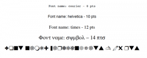
The PyFPDF has a set of core fonts hard-coded into its FPDF class:

self.core_fonts={'courier': 'Courier',
    'courierB': 'Courier-Bold',
    'courierBI': 'Courier-BoldOblique',
    'courierI': 'Courier-Oblique',
    'helvetica': 'Helvetica',
    'helveticaB': 'Helvetica-Bold', 
    'helveticaBI': 'Helvetica-BoldOblique',
    'helveticaI': 'Helvetica-Oblique',
    'symbol': 'Symbol',
    'times': 'Times-Roman',
    'timesB': 'Times-Bold',
    'timesBI': 'Times-BoldItalic',
    'timesI': 'Times-Italic',
    'zapfdingbats': 'ZapfDingbats'}

You will note that Arial is not listed here even though we used it in the previous example. Arial is getting remapped to Helvetica in the actual source code, so you are not really using Arial at all. Anyway, let’s learn how you can change fonts using PyFPDF:

# change_fonts.py 
from fpdf import FPDF
 
def change_fonts():
    pdf = FPDF()
    pdf.add_page()
    font_size = 8for font in pdf.core_fonts:
        if any([letter for letter in font if letter.isupper()]):
            # skip this fontcontinue
        pdf.set_font(font, size=font_size)
        txt = "Font name: {} - {} pts".format(font, font_size)
        pdf.cell(0, 10, txt=txt, ln=1, align="C")
        font_size += 2 
    pdf.output("change_fonts.pdf") 
if __name__ == '__main__':
    change_fonts()

Here we create a simple function called change_fonts and then we create an instance of the FPDF class. The next step is to create a page and then loop over the core fonts. When I tried that, I discovered that PyFPDF doesn’t consider the variant names of its core fonts as valid fonts (i.e. helveticaB, helveticaBI, etc). So to skip those variants, we create a list comprehension and check for any capital characters in the font’s name. If there is one, we skip that font. Otherwise we set the font and the font size and write it out. We also increase the font size by two points each time through the loop. If you want to change the font’s color, then you can call set_text_color and pass in the RGB value that you require.

The result of running this code looks like this:

I like how easy it is to change fonts in PyFPDF. However the number of core fonts is pretty small. You can add TrueType, OpenType or Type1 fonts using PyFPDF though via the add_font method. This method takes the following arguments:

  • family (font family)
  • style (font style)
  • fname (font file name or full path to font file)
  • uni (TTF Unicode flag)

The example that PyFPDF’s documentation uses is as follows:

pdf.add_font('DejaVu', '', 'DejaVuSansCondensed.ttf', uni=True)

You would call **add_font** before attempting to use it via the **set_font** method. I tried this on Windows and got an error as Windows couldn’t find this font, which is what I expected. This is a really simply way to add fonts though and will probably work. Note that it uses the following search paths:

  • FPDF_FONTPATH
  • SYSTEM_TTFONTS

These appear to be constants that are defined either in your environment or in the PyFPDF package itself. The documentation does not explain how these are set or modified however, if you look closely at the API and the source code, it would appear that you would have to do the following at the beginning of your code:

import fpdf
 
fpdf.SYSTEM_TTFONTS = '/path/to/system/fonts'

The SYSTEM_TTFONTS is set to None by default otherwise.


Drawing

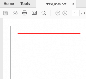
The PyFPDF package has limited drawing support. You can draw lines, ellipses and rectangles. Let’s take a look at how to draw lines first:

# draw_lines.py 
from fpdf import FPDF
 
def draw_lines():
    pdf = FPDF()
    pdf.add_page()
    pdf.line(10, 10, 10, 100)
    pdf.set_line_width(1)
    pdf.set_draw_color(255, 0, 0)
    pdf.line(20, 20, 100, 20)
    pdf.output('draw_lines.pdf') 
if __name__ == '__main__':
    draw_lines()

Here we call the line method and pass it two pairs of x/y coordinates. The line width defaults to 0.2 mm so we increase it to 1 mm for the second line by calling the set_line_width method. We also set the color of the second line by calling set_draw_color to an RGB value equivalent to red. The output looks like this:

Now we can move on and draw a couple of shapes:

# draw_shapes.py 
from fpdf import FPDF
 
def draw_shapes():
    pdf = FPDF()
    pdf.add_page()
    pdf.set_fill_color(255, 0, 0)
    pdf.ellipse(10, 10, 10, 100, 'F') 
    pdf.set_line_width(1)
    pdf.set_fill_color(0, 255, 0)
    pdf.rect(20, 20, 100, 50)
    pdf.output('draw_shapes.pdf') 
if __name__ == '__main__':
    draw_shapes()

When you draw a shape like an ellipse or a rect, you will need to pass in the x and y coordinates that represent the upper left corner of the drawing. Then you will want to pass in the width and height of the shape. The last argument you can pass in is for style which can be “D” or an empty string (default), “F” for fill or “DF” for draw and fill. In this example, we fill the ellipse and use the default for the rectangle. The result ends up looking like this:

Now let’s learn about image support.


Adding Images

The PyFPDF package supports adding JPEG, PNG and GIF formats to your PDF. If you happen to try to use an animated GIF, only the first frame is used. Also of note is that if you add the same image multiple times to the document, PyFPDF is smart enough to only embed one actual copy of the image. Here is a very simple example of adding an image to a PDF using PyFPDF:

# add_image.py 
from fpdf import FPDF
 
def add_image(image_path):
    pdf = FPDF()
    pdf.add_page()
    pdf.image(image_path, x=10, y=8, w=100)
    pdf.set_font("Arial", size=12)
    pdf.ln(85)# move 85 down
    pdf.cell(200, 10, txt="{}".format(image_path), ln=1)
    pdf.output("add_image.pdf") 
if __name__ == '__main__':
    add_image('snakehead.jpg')

The new piece of code here is the call to the image method. Its signature looks like the this:

image(name, x = None, y = None, w = 0, h = 0, type = '', link = '')

You specify the image file path, the x and y coordinate and the width and height. If you only specify the width or the height, the other is calculated for you and attempts to maintain the original proportions of the image. You can also specify the file type explicitly, otherwise it is guessed from the file name. Finally you can add a link / URL when adding the image.

When you run this code, you should see something like the following:

Now let’s learn how PyFPDF supports doing multipage documents.


Multipage Documents

PyFPDF had multipage support enabled by default. If you add enough cells to a page, it will automatically create a new page and continue to add your new text to the next page. Here is a simple example:

# multipage_simple.py 
from fpdf import FPDF
 
def multipage_simple():
    pdf = FPDF()
    pdf.set_font("Arial", size=12)
    pdf.add_page()
    line_no = 1for i inrange(100):
        pdf.cell(0, 10, txt="Line #{}".format(line_no), ln=1)
        line_no += 1
    pdf.output("multipage_simple.pdf") 
if __name__ == '__main__':
    multipage_simple()

All this does is create 100 lines of text. When I ran this code, I ended up with a PDF that contained 4 pages of text.


Headers and Footers

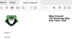
The PyFPDF package has built-in support for adding headers, footers and page numbers. The FPDF class just needs to be sub-classed and the the header and footer methods overridden to make them work. Let’s take a look:

# header_footer.py 
from fpdf import FPDF
 
class CustomPDF(FPDF):
 
    def header(self):
        # Set up a logoself.image('snakehead.jpg', 10, 8, 33)self.set_font('Arial', 'B', 15) 
        # Add an addressself.cell(100)self.cell(0, 5, 'Mike Driscoll', ln=1)self.cell(100)self.cell(0, 5, '123 American Way', ln=1)self.cell(100)self.cell(0, 5, 'Any Town, USA', ln=1) 
        # Line breakself.ln(20) 
    def footer(self):
        self.set_y(-10) 
        self.set_font('Arial', 'I', 8) 
        # Add a page number
        page = 'Page ' + str(self.page_no()) + '/{nb}'self.cell(0, 10, page, 0, 0, 'C') 
def create_pdf(pdf_path):
    pdf = CustomPDF()# Create the special value {nb}
    pdf.alias_nb_pages()
    pdf.add_page()
    pdf.set_font('Times', '', 12)
    line_no = 1for i inrange(50):
        pdf.cell(0, 10, txt="Line #{}".format(line_no), ln=1)
        line_no += 1
    pdf.output(pdf_path) 
if __name__ == '__main__':
    create_pdf('header_footer.pdf')

Since this is a fairly long piece of code, let’s go over this piece-by-piece. The first section that we want to look at is the header method:

def header(self):
    # Set up a logoself.image('snakehead.jpg', 10, 8, 33)self.set_font('Arial', 'B', 15) 
    # Add an addressself.cell(100)self.cell(0, 5, 'Mike Driscoll', ln=1)self.cell(100)self.cell(0, 5, '123 American Way', ln=1)self.cell(100)self.cell(0, 5, 'Any Town, USA', ln=1) 
    # Line breakself.ln(20)

Here we just hard-code in the logo image that we want to use and then we set the font that we will be using in our header. Next we add an address and we position that address to the right of the image. You will notice that when you are using PyFPDF, the origin is the top left of the page. So if we want to move our text over to the right, then we need to create a cell with a number of units of measurement. In this case, we move the next three lines over to the right by adding a cell of 100 mm. Then we add a line break at the end, which should add 20 mm of vertical space.

Next up, we want to override the footer method:

def footer(self):
    self.set_y(-10) 
    self.set_font('Arial', 'I', 8) 
    # Add a page number
    page = 'Page ' + str(self.page_no()) + '/{nb}'self.cell(0, 10, page, 0, 0, 'C')

The first thing we do here is set the y-position of the origin on the page to -10 mm or -1 cm. This puts the footer’s origin right above the bottom of the page. Then we set our font for the footer. Finally we create the page number text. You will note the reference to {nb}. This is a special value in PyFPDF that is inserted when you call alias_nb_pages and represents the total number of pages in the document. The last step in the footer is to write the page text on the page and center it.

The final piece of code to look at is in the create_pdf function:

def create_pdf(pdf_path):
    pdf = CustomPDF()# Create the special value {nb}
    pdf.alias_nb_pages()
    pdf.add_page()
    pdf.set_font('Times', '', 12)
    line_no = 1for i inrange(50):
        pdf.cell(0, 10, txt="Line #{}".format(line_no), ln=1)
        line_no += 1
    pdf.output(pdf_path)

This is where we call the somewhat magical **alias_nb_pages** method that will help us get the total number of pages. We also set the font for the portion of the page that is not taken up by the header or footer. Then we write 50 lines of text to the document to make it create a multipage PDF.

When you run this code you should see a page that looks something like this:

Now let’s find out how you can create tables with PyFPDF.


Tables

The PyFPDF does not have a table control. Instead you have to build your tables using cells or HTML. Let’s take a look at how you might create a table using cells first:

# simple_table.py 
from fpdf import FPDF
 
def simple_table(spacing=1):
    data = [['First Name', 'Last Name', 'email', 'zip'],
            ['Mike', 'Driscoll', 'mike@somewhere.com', '55555'],
            ['John', 'Doe', 'jdoe@doe.com', '12345'],
            ['Nina', 'Ma', 'inane@where.com', '54321']] 
    pdf = FPDF()
    pdf.set_font("Arial", size=12)
    pdf.add_page() 
    col_width = pdf.w / 4.5
    row_height = pdf.font_sizefor row in data:
        for item in row:
            pdf.cell(col_width, row_height*spacing,
                     txt=item, border=1)
        pdf.ln(row_height*spacing) 
    pdf.output('simple_table.pdf') 
if __name__ == '__main__':
    simple_table()

Here we just create a simple list of lists and then loop over it. For each row in the list and each element in the nested row, we add a cell to our PDF object. Note that we turn the border on for these cells. When we finish iterating over a row, we add a linebreak. If you want the cells to have more space in the cells, then you can pass in a spacing value. When I ran this script, I ended up with a table that looked like this:

This is a pretty crude way to create tables though. I personally prefer ReportLab’s methodology here.

The alternative method is to use HTML to create your table:

# simple_table_html.py 
from fpdf import FPDF, HTMLMixin
 
class HTML2PDF(FPDF, HTMLMixin):
    pass 
def simple_table_html():
    pdf = HTML2PDF() 
    table = """<table border="0" align="center" width="50%">
    <thead><tr><th width="30%">Header 1</th><th width="70%">header 2</th></tr></thead>
    <tbody>
    <tr><td>cell 1</td><td>cell 2</td></tr>
    <tr><td>cell 2</td><td>cell 3</td></tr>
    </tbody>
    </table>""" 
    pdf.add_page()
    pdf.write_html(table)
    pdf.output('simple_table_html.pdf') 
if __name__ == '__main__':
    simple_table_html()

Here we use PyFPDF’s HTMLMixin class to allow it to accept HTML as an input and transform that into a PDF. When you run this example, you will end up with the following:

There are some examples on the website that use the Web2Py framework in conjunction with PyFPDF to create better looking tables, but the code was incomplete so I won’t be demonstrating that here.


Transform HTML to PDF

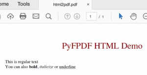
The PyFDPF package has some limited support for HTML tags. You can create headings, paragraphs and basic text styling using HTML. You can also add hyperlinks, images, lists and tables. Check the documentation for the full list of tags and attributes that are supported. You can then take basic HTML and turn it into a PDF using the HTMLMixin that we saw in the previous section when we created our table.

# html2fpdf.py 
from fpdf import FPDF, HTMLMixin
 
class HTML2PDF(FPDF, HTMLMixin):
    pass 
def html2pdf():
    html = '''<h1 align="center">PyFPDF HTML Demo</h1>
    <p>This is regular text</p>
    <p>You can also <b>bold</b>, <i>italicize</i> or <u>underline</u>
    '''
    pdf = HTML2PDF()
    pdf.add_page()
    pdf.write_html(html)
    pdf.output('html2pdf.pdf') 
if __name__ == '__main__':
    html2pdf()

Here we just use pretty standard HTML markup to design the PDF. It actually ends up looking pretty good when you run this code:


Web2Py

The Web2Py framework includes PyFPDF package to make creating reports in the framework easier. This allows you to create PDF templates in Web2Py. The documentation is a bit scarce on this subject, so I won’t be covering this subject in this book. However it does appear that you can do halfway decent reports using Web2Py this way.


Templates

You can also create templates using PyFPDF. The package even includes a designer script that uses wxPython for its user interface. The templates that you can create would be where you want to specify where each element appears on the page, its style (font, size, etc) and the default text to use. The templating system supports using CSV files or databases. There is only one example in the documentation on this subject though, which is a bit disappointing. While I do think this part of the library holds promise, due to the lack of documentation, I don’t feel comfortable writing about it extensively.


Wrapping Up

The PyFPDF package is a fairly nice project that let’s you do basic PDF generation. They do point out in the FAQ that they do not support charts or widgets or a “flexible page layout system” like ReportLab. They also do not support PDF text extraction or conversion like PDFMiner or PyPDF2. However if all you need are the bare bone basics to generate a PDF, then this library might work for you. I think its learning curve is simpler than ReportLab’s is. However PyFPDF is nowhere near as feature-rich as ReportLab and I didn’t feel like you had quite the same granularity of control when it came to placing elements on the page.


Related Reading


Source Code

Python Bytes: #81 Making your C library callable from Python by wrapping it with Cython

Red Hat Developers: How to install Python Flask on Red Hat Enterprise Linux 7

$
0
0

I recently got my zero-dollar developer copy of Red Hat Enterprise Linux (RHEL, version 7.5) and built a virtual machine (VM) to run it. There it was, on my PC, running in VirtualBox…a gleaming, shiny, brand-spanking-new VM running RHEL. Whatever shall I do with it?

Then I got the idea: I’ll install the Red Hat Container Development Kit (CDK) and build some Python-based containers. I’ll use Flask, a terrific microframework that makes building RESTful services easy.

But I don’t have RHEL 7.5

If you aren’t using RHEL 7.5, not to worry. Because Python 3 is part of the Red Hat Software Collections (RHSCL), this works with all minor versions of RHEL 7.

I Mean…Obviously…

Obviously, installing Flask would be easy. With the confidence that often accompanies ignorance, I went to the command line and typed the simple command pip install flask and waited for the good news.

Oops.

RHEL is Yummy

Well, hang on a minute; I’m on RHEL, so yum is the package manager (that is, installation utility). Obviously, the correct command is sudo yum install pip.

yum search to the Rescue

Frustrated, but not to be defeated, I figured pipa Python utility—must be part of the Python package for RHEL. I used the command yum search python36 to see if any Python 3.6 packages were available, and voila!

Aha! A package specifically built by Red Hat. Finally, the install command I was looking for: sudo yum install rh-python36-python-pip.noarch.

I’m An Enabler

Now, all I needed to do was enable it in a bash shell session and I’d be ready to start writing Python code using Flask:

sudo scl enable rh-python36 bash

I then immediately ran pip install --upgrade pip and my pip installation was updated to version pip-10.0.1.

Ready for Flask

Now, finally, I could install Flask by running pip install flask.

Success!

Finally—for real this time—I tested it by creating and running the hello.py app that’s featured on the Flask project home page. It worked.

Onward!

I now have Python 3.6 and Flask installed on my RHEL VM. All I need to do now is to install the CDK and I can start building Python microservices.


Share

The post How to install Python Flask on Red Hat Enterprise Linux 7 appeared first on RHD Blog.


Python Does What?!: when no-ops attack VII: assignment's revenge

$
0
0
Let's define a very simple class:

>>> class F(object):
...    @staticmethod
...    def f(): return "I'm such a simple function, nothing could go wrong"
...

>>> F.f()
"I'm such a simple function, nothing could go wrong"


 Now, let's do a trivial no-op to this class:

>>> F.f = F.f

Surely nothing changed, right?

>>> F.f()
Traceback (most recent call last):
  File "<stdin>", line 1, in <module>
TypeError: unbound method f() must be called with F instance as first argument (got nothing instead)


What happened?  staticmethod uses the descriptor protocol in order to return something other than itself when accessed as an attribute.  The assignment above is not a no-op, because it is not setting the value back to what it already was, but to what was returned by __get__ of the staticmethod object.

>>> class F(object):
...    @staticmethod
...    def f(): return "I'm not what I seem"
...
>>> F.f

<function f at 0x7f05eda596e0>
>>> F.__dict__['f']
<staticmethod object at 0x7f05eda5ce50>

Version note -- Python3 doesn't raise an exception, although the type still changes from staticmethod to function.

>>> class F:
...    @staticmethod
...    def f(): return "I'm protected by python3 wizardry"
...
>>> F.f()
"I'm protected by python3 wizardry"
>>> F.__dict__['f']
<staticmethod object at 0x7fd087b739b0>
>>> F.f = F.f
>>> F.__dict__['f']
<function F.f at 0x7fd087b5cae8>
>>> F.f()
"I'm protected by python3 wizardry"

Real Python: Basic Data Types in Python

$
0
0

Now you know how to interact with the Python interpreter and execute Python code. It’s time to dig into the Python language. First up is a discussion of the basic data types that are built into Python.

Here’s what you’ll learn in this tutorial:

  • You’ll learn about several basic numeric, string, and Boolean types that are built into Python. By the end of this tutorial, you’ll be familiar with what objects of these types look like, and how to represent them.
  • You’ll also get an overview of Python’s built-in functions. These are pre-written chunks of code you can call to do useful things. You have already seen the built-in print() function, but there are many others.

Get Notified: Don't miss the follow up to this tutorial—Click here to join the Real Python Newsletter and you'll know when the next instalment comes out.

Integers

In Python 3, there is effectively no limit to how long an integer value can be. Of course, it is constrained by the amount of memory your system has, as are all things, but beyond that an integer can be as long as you need it to be:

>>> print(123123123123123123123123123123123123123123123123+1)123123123123123123123123123123123123123123123124

Python interprets a sequence of decimal digits without any prefix to be a decimal number:

>>> print(10)10

The following strings can be prepended to an integer value to indicate a base other than 10:

PrefixInterpretationBase
0b (zero + lowercase letter 'b')
0B (zero + uppercase letter 'B')
Binary2
0o (zero + lowercase letter 'o')
0O (zero + uppercase letter 'O')
Octal8
0x (zero + lowercase letter 'x')
0X (zero + uppercase letter 'X')
Hexadecimal16

For example:

>>> print(0o10)8>>> print(0x10)16>>> print(0b10)2

For more information on integer values with non-decimal bases, see the following Wikipedia sites: Binary, Octal, and Hexadecimal.

The underlying type of a Python integer, irrespective of the base used to specify it, is called int:

>>> type(10)<class 'int'>>>> type(0o10)<class 'int'>>>> type(0x10)<class 'int'>

Note: This is a good time to mention that if you want to display a value while in a REPL session, you don’t need to use the print() function. Just typing the value at the >>> prompt and hitting Enter will display it:

>>> 1010>>> 0x1016>>> 0b102

Many of the examples in this tutorial series will use this feature.

Note that this does not work inside a script file. A value appearing on a line by itself in a script file will not do anything.

Floating-Point Numbers

The float type in Python designates a floating-point number. float values are specified with a decimal point. Optionally, the character e or E followed by a positive or negative integer may be appended to specify scientific notation:

>>> 4.24.2>>> type(4.2)<class 'float'>>>> 4.4.0>>> .20.2>>> .4e74000000.0>>> type(.4e7)<class 'float'>>>> 4.2e-40.00042

Deep Dive: Floating-Point Representation

The following is a bit more in-depth information on how Python represents floating-point numbers internally. You can readily use floating-point numbers in Python without understanding them to this level, so don’t worry if this seems overly complicated. The information is presented here in case you are curious.

Almost all platforms represent Python float values as 64-bit “double-precision” values, according to the IEEE 754 standard. In that case, the maximum value a floating-point number can have is approximately 1.8 ⨉ 10308. Python will indicate a number greater than that by the string inf:

1.79e3081.79e+3081.8e308inf

The closest a nonzero number can be to zero is approximately 5.0 ⨉ 10-324. Anything closer to zero than that is effectively zero:

5e-3245e-3241e-3250.0

Floating point numbers are represented internally as binary (base-2) fractions. Most decimal fractions cannot be represented exactly as binary fractions, so in most cases the internal representation of a floating-point number is an approximation of the actual value. In practice, the difference between the actual value and the represented value is very small and should not usually cause significant problems.

Further Reading: For additional information on floating-point representation in Python and the potential pitfalls involved, see Floating Point Arithmetic: Issues and Limitations in the Python documentation.

Complex Numbers

Complex numbers are specified as <real part>+<imaginary part>j. For example:

>>> 2+3j(2+3j)>>> type(2+3j)<class 'complex'>

Strings

Strings are sequences of character data. The string type in Python is called str.

String literals may be delimited using either single or double quotes. All the characters between the opening delimiter and matching closing delimiter are part of the string:

>>> print("I am a string.")I am a string.>>> type("I am a string.")<class 'str'>>>> print('I am too.')I am too.>>> type('I am too.')<class 'str'>

A string in Python can contain as many characters as you wish. The only limit is your machine’s memory resources. A string can also be empty:

>>> ''''

What if you want to include a quote character as part of the string itself? Your first impulse might be to try something like this:

>>> print('This string contains a single quote (')character.')SyntaxError: invalid syntax

As you can see, that doesn’t work so well. The string in this example opens with a single quote, so Python assumes the next single quote, the one in parentheses which was intended to be part of the string, is the closing delimiter. The final single quote is then a stray and causes the syntax error shown.

If you want to include either type of quote character within the string, the simplest way is to delimit the string with the other type. If a string is to contain a single quote, delimit it with double quotes and vice versa:

>>> print("This string contains a single quote (') character.")This string contains a single quote (') character.>>> print('This string contains a double quote (") character.')This string contains a double quote (") character.

Escape Sequences in Strings

Sometimes, you want Python to interpret a character or sequence of characters within a string differently. This may occur in one of two ways:

  • You may want to suppress the special interpretation that certain characters are usually given within a string.
  • You may want to apply special interpretation to characters in a string which would normally be taken literally.

You can accomplish this using a backslash (\) character. A backslash character in a string indicates that one or more characters that follow it should be treated specially. (This is referred to as an escape sequence, because the backslash causes the subsequent character sequence to “escape” its usual meaning.)

Let’s see how this works.

Suppressing Special Character Meaning

You have already seen the problems you can come up against when you try to include quote characters in a string. If a string is delimited by single quotes, you can’t directly specify a single quote character as part of the string because, for that string, the single quote has special meaning—it terminates the string:

>>> print('This string contains a single quote (')character.')SyntaxError: invalid syntax

Specifying a backslash in front of the quote character in a string “escapes” it and causes Python to suppress its usual special meaning. It is then interpreted simply as a literal single quote character:

>>> print('This string contains a single quote (\') character.')This string contains a single quote (') character.

The same works in a string delimited by double quotes as well:

>>> print("This string contains a double quote (\") character.")This string contains a double quote (") character.

The following is a table of escape sequences which cause Python to suppress the usual special interpretation of a character in a string:

Escape
Sequence
Usual Interpretation of
Character(s) After Backslash
“Escaped” Interpretation
\'Terminates string with single quote opening delimiterLiteral single quote (') character
\"Terminates string with double quote opening delimiterLiteral double quote (") character
\newlineTerminates input lineNewline is ignored
\\Introduces escape sequenceLiteral backslash (\) character

Ordinarily, a newline character terminates line input. So pressing Enter in the middle of a string will cause Python to think it is incomplete:

>>> print('aSyntaxError: EOL while scanning string literal

To break up a string over more than one line, include a backslash before each newline, and the newlines will be ignored:

>>> print('a\... b\... c')abc

To include a literal backslash in a string, escape it with a backslash:

>>> print('foo\\bar')foo\bar

Applying Special Meaning to Characters

Next, suppose you need to create a string that contains a tab character in it. Some text editors may allow you to insert a tab character directly into your code. But many programmers consider that poor practice, for several reasons:

  • The computer can distinguish between a tab character and a sequence of space characters, but you can’t. To a human reading the code, tab and space characters are visually indistinguishable.
  • Some text editors are configured to automatically eliminate tab characters by expanding them to the appropriate number of spaces.
  • Some Python REPL environments will not insert tabs into code.

In Python (and almost all other common computer languages), a tab character can be specified by the escape sequence \t:

>>> print('foo\tbar')foo     bar

The escape sequence \t causes the t character to lose its usual meaning, that of a literal t. Instead, the combination is interpreted as a tab character.

Here is a list of escape sequences that cause Python to apply special meaning instead of interpreting literally:

Escape Sequence“Escaped” Interpretation
\aASCII Bell (BEL) character
\bASCII Backspace (BS) character
\fASCII Formfeed (FF) character
\nASCII Linefeed (LF) character
\N{<name>}Character from Unicode database with given <name>
\rASCII Carriage Return (CR) character
\tASCII Horizontal Tab (TAB) character
\uxxxxUnicode character with 16-bit hex value xxxx
\UxxxxxxxxUnicode character with 32-bit hex value xxxxxxxx
\vASCII Vertical Tab (VT) character
\oooCharacter with octal value ooo
\xhhCharacter with hex value hh

Examples:

>>> print("a\tb")a    b>>> print("a\141\x61")aaa>>> print("a\nb")ab>>> print('\u2192\N{rightwards arrow}')→ →

This type of escape sequence is typically used to insert characters that are not readily generated from the keyboard or are not easily readable or printable.

Raw Strings

A raw string literal is preceded by r or R, which specifies that escape sequences in the associated string are not translated. The backslash character is left in the string:

>>> print('foo\nbar')foobar>>> print(r'foo\nbar')foo\nbar>>> print('foo\\bar')foo\bar>>> print(R'foo\\bar')foo\\bar

Triple-Quoted Strings

There is yet another way of delimiting strings in Python. Triple-quoted strings are delimited by matching groups of three single quotes or three double quotes. Escape sequences still work in triple-quoted strings, but single quotes, double quotes, and newlines can be included without escaping them. This provides a convenient way to create a string with both single and double quotes in it:

>>> print('''This string has a single (') and a double (") quote.''')This string has a single (') and a double (") quote.

Because newlines can be included without escaping them, this also allows for multiline strings:

>>> print("""This is astring that spansacross several lines""")This is astring that spansacross several lines

You will see in the upcoming tutorial on Python Program Structure how triple-quoted strings can be used to add an explanatory comment to Python code.

Boolean Type, Boolean Context, and “Truthiness”

Python 3 provides a Boolean data type. Objects of Boolean type may have one of two values, True or False:

>>> type(True)<class 'bool'>>>> type(False)<class 'bool'>

As you will see in upcoming tutorials, expressions in Python are often evaluated in Boolean context, meaning they are interpreted to represent truth or falsehood. A value that is true in Boolean context is sometimes said to be “truthy,” and one that is false in Boolean context is said to be “falsy.” (You may also see “falsy” spelled “falsey.”)

The “truthiness” of an object of Boolean type is self-evident: Boolean objects that are equal to True are truthy (true), and those equal to False are falsy (false). But non-Boolean objects can be evaluated in Boolean context as well and determined to be true or false.

You will learn more about evaluation of objects in Boolean context when you encounter logical operators in the upcoming tutorial on operators and expressions in Python.

Built-In Functions

The Python interpreter supports many functions that are built-in: sixty-eight, as of Python 3.6. You will cover many of these in the following discussions, as they come up in context.

For now, a brief overview follows, just to give a feel for what is available. See the Python documentation on built-in functions for more detail. Many of the following descriptions refer to topics and concepts that will be discussed in future tutorials.

Math

FunctionDescription
abs()Returns absolute value of a number
divmod()Returns quotient and remainder of integer division
max()Returns the largest of the given arguments or items in an iterable
min()Returns the smallest of the given arguments or items in an iterable
pow()Raises a number to a power
round()Rounds a floating-point value
sum()Sums the items of an iterable

Type Conversion

FunctionDescription
ascii()Returns a string containing a printable representation of an object
bin()Converts an integer to a binary string
bool()Converts an argument to a Boolean value
chr()Returns string representation of character given by integer argument
complex()Returns a complex number constructed from arguments
float()Returns a floating-point object constructed from a number or string
hex()Converts an integer to a hexadecimal string
int()Returns an integer object constructed from a number or string
oct()Converts an integer to an octal string
ord()Returns integer representation of a character
repr()Returns a string containing a printable representation of an object
str()Returns a string version of an object
type()Returns the type of an object or creates a new type object

Iterables and Iterators

FunctionDescription
all()Returns True if all elements of an iterable are true
any()Returns True if any elements of an iterable are true
enumerate()Returns a list of tuples containing indices and values from an iterable
filter()Filters elements from an iterable
iter()Returns an iterator object
len()Returns the length of an object
map()Applies a function to every item of an iterable
next()Retrieves the next item from an iterator
range()Generates a range of integer values
reversed()Returns a reverse iterator
slice()Returns a slice object
sorted()Returns a sorted list from an iterable
zip()Creates an iterator that aggregates elements from iterables

Composite Data Type

FunctionDescription
bytearray()Creates and returns an object of the bytearray class
bytes()Creates and returns a bytes object (similar to bytearray, but immutable)
dict()Creates a dict object
frozenset()Creates a frozenset object
list()Constructs a list object
object()Returns a new featureless object
set()Creates a set object
tuple()Creates a tuple object

Classes, Attributes, and Inheritance

FunctionDescription
classmethod()Returns a class method for a function
delattr()Deletes an attribute from an object
getattr()Returns the value of a named attribute of an object
hasattr()Returns True if an object has a given attribute
isinstance()Determines whether an object is an instance of a given class
issubclass()Determines whether a class is a subclass of a given class
property()Returns a property value of a class
setattr()Sets the value of a named attribute of an object
super()Returns a proxy object that delegates method calls to a parent or sibling class

Input/Output

FunctionDescription
format()Converts a value to a formatted representation
input()Reads input from the console
open()Opens a file and returns a file object
print()Prints to a text stream or the console

Variables, References, and Scope

FunctionDescription
dir()Returns a list of names in current local scope or a list of object attributes
globals()Returns a dictionary representing the current global symbol table
id()Returns the identity of an object
locals()Updates and returns a dictionary representing current local symbol table
vars()Returns __dict__ attribute for a module, class, or object

Miscellaneous

FunctionDescription
callable()Returns True if object appears callable
compile()Compiles source into a code or AST object
eval()Evaluates a Python expression
exec()Implements dynamic execution of Python code
hash()Returns the hash value of an object
help()Invokes the built-in help system
memoryview()Returns a memory view object
staticmethod()Returns a static method for a function
__import__()Invoked by the import statement

Conclusion

In this tutorial, you learned about the built-in data types and functions Python provides.

The examples given so far have all manipulated and displayed only constant values. In most programs, you are usually going to want to create objects that change in value as the program executes.

Head to the next tutorial to learn about Python variables.

Get Notified: Don't miss the follow up to this tutorial—Click here to join the Real Python Newsletter and you'll know when the next instalment comes out.


[ Improve Your Python With 🐍 Python Tricks 💌 – Get a short & sweet Python Trick delivered to your inbox every couple of days. >> Click here to learn more and see examples ]

NumFOCUS: Meet the NumFOCUS Google Summer of Code 2018 Cohort

Python Engineering at Microsoft: Python in Visual Studio Code – May 2018 Release

$
0
0

We are pleased to announce that the May 2018 release of the Python Extension for Visual Studio Code is now available from the marketplace and the gallery. You can download the Python extension from the marketplace, or install it directly from the extension gallery in Visual Studio Code. You can learn more about Python support in Visual Studio Code in the VS Code documentation.

In this release we have closed a total of 103 issues including support for the new and popular formatter Black, improvements to the experimental debugger and formatting as you type.

Support for Black Formatter

Black is a new code formatting tool for Python that was first released in March and has quickly gained popularity. Black has a single opinion about how Python code should be formatted, allowing you to easily achieve consistency across your codebase. The Python extension now supports using it as a formatter.

To enable the Black formatter, go into File > User Preferences > Settings, and put the following setting in your User Settings (for settings for all workspaces) or Workspace settings (for the current workspace/folder).

"python.formatting.provider": "black"

Then run the VS Code command “Format Document”. You will get a prompt to install the Black formatter:

Selecting Yes will install Black into the currently selected interpreter in VS Code. Once Black has finished installing, you will need to run the Format Document command again to format your document.

In the below code example, we can see that black adds a blank line before functions, spaces around equals signs, and uses double quotation marks instead of single quotation marks:

If you want formatting to happen automatically when hitting save, you can add the following setting:

"editor.formatOnSave": true

If you want to format Python 2.7 code, Black will need to run in a Python 3 environment. In that case, you can install black using python3 –m pip install –upgrade black into a Python 3 interpreter/environment of your choice, and then set the python.formatting.blackPath setting to point to the black command that was installed (on UNIX-based OSs you can typically find this with the command which black).

Various Fixes and Enhancements

We have also added small enhancements and fixed issues requested by users that should improve your experience working with Python in Visual Studio Code. The full list of improvements is listed in our changelog, some notable improvements are:

  1. Improvements to testing: added a ‘Discover Unit Tests’ command (#1474) for discovering unit tests, removed error in the output window when running tests (#1529)
  2. Improvements to the Experimental Debugger: auto-enable jinja template debugging on *.jinja and *.j2 files (#1484), ensure debugged program is terminated when Stop debugging button is clicked. (#1345), support for attach/detach (#1255)
  3. Fixed syntax errors caused when using the editor.formatOnType setting is enabled (#1799)
  4. Ensure python environment activation works as expected within a multi-root workspace. (#1476)
  5. Fixed flask debugging configurations so that they work with the latest versions of flask (#1634)
  6. Ensure the display name of an interpreter does not get prefixed twice with the words Python. (#1651)
  7. `Go to Definition` now works for functions which have numbers that use `_` as a separator (as part of our Jedi 0.12.0 upgrade). (#180)
  8. Fixed rename refactor issue that removes the last line of the source file when the line is being refactored and source does not end with an EOL. (#695)

Be sure to download the Python extension for VS Code now to try out the above improvements. If you run into any issues be sure to file an issue on the Python VS Code GitHub page.

Techiediaries - Django: Angular 6 Tutorial with Django RESTful API — Building Bootstrap 4 UIs

$
0
0

In this Angular 6 tutorial we'll learn how to use Bootstrap 4 with Angular 6 to build professional UIs.

Angular 6 is the latest version of Angular when writing this tutorial and Bootstrap 4 is the latest version of Bootstrap — The most popular CSS framework. You can use Bootstrap to create professional looking interfaces without being a CSS designer.

In this tutorial, we'll particularly look at how to add Bootstrap 4 to Angular projects generated using Angular CLI 6.

In the previous tutorial, we've built a web application with Angular 6 and Django. In this part, we're going to style the UI interface with Bootstrap 4, after installing and setting up the framework in the Angular 6 front-end.

In the previous tutorial we’ve: - Installed Angular CLI v6. - Generated a new front-end application using Angular CLI v6. - Created some UI components.

In this tutorial, we'll be using the following versions of libraries:

  • Angular 6 and Angular CLI 6.
  • Bootstrap 4.

Different Ways to Integrate Bootstrap 4 with Angular 6

There are many ways to add Bootstrap 4 to Angular 6 projects:

  • Installing bootstrap and jquery via npm and add adding scripts and styles to angular.json.
  • Importing bootstrap style and script files in src/index.html. You can use a bootstrap 4 CDN.
  • Installing bootstrap via npm and importing @import "~bootstrap/dist/css/bootstrap.css"; in src/styles.css.
  • Installing and using ng-bootstrap npm install --save @ng-bootstrap/ng-bootstrap: It's a library that contains native Angular components for Bootstrap’s markup and CSS styles. It's not dependent on jQuery or Bootstrap’s JavaScript.

How to Work with This Tutorial?

To complete this tutorial, you'll need to, either:

  • Start with the previous tutorial, which takes you from installing the Angular CLI 6 to calling the Django RESTful API
  • Clone the font-end project from GitHub and follow the steps in the previous tutorial for setting up the project.
  • Directly follow the steps to integrate Bootstrap 4 in your own Angular 6 project.

How to add Bootstrap 4 to your Angular 6 Front-End?

After seeing different ways to add Bootstrap 4 to Angular 6, let's now style our Angular 6 front-end UI, built in the previous tutorial, with Bootstrap. We'll use the first approach i.e we'll install bootstrap from npm and then we'll include bootstrap.css CSS file, jQuery and Popover.js

Please note that projects generated using Angular CLI 6 are using angular.json instead of .angular-cli.json for configuration settings

Installing Bootstrap 4 and jQuery

Head over to your project, you created in the previous tutorial, navigate inside your Angular 6 front-end application:

cd frontend

Next, install bootstrap and jquery from npm using:

npm install --save bootstrap jquery

Adding Bootstrap 4 to Angular CLI v6

Next, open angular.json. You should similar content to the following:

{"$schema":"./node_modules/@angular/cli/lib/config/schema.json","version":1,"newProjectRoot":"projects","projects":{"crmapp":{"root":"","sourceRoot":"src","projectType":"application","prefix":"app","schematics":{},"architect":{"build":{"builder":"@angular-devkit/build-angular:browser","options":{"outputPath":"dist/crmapp","index":"src/index.html","main":"src/main.ts","polyfills":"src/polyfills.ts","tsConfig":"src/tsconfig.app.json","assets":["src/favicon.ico","src/assets"],"styles":["src/styles.css"],"scripts":[]},...},"defaultProject":"crmapp"}

Under projects -> architect -> build -> scripts add node_modules/jquery/dist/jquery.min.js and node_modules/bootstrap/dist/js/bootstrap.min.js:

"scripts":["node_modules/jquery/dist/jquery.min.js","node_modules/bootstrap/dist/js/bootstrap.min.js"]

Under projects -> architect -> build -> styles add node_modules/bootstrap/dist/css/bootstrap.min.css:

"styles":["src/styles.css","node_modules/bootstrap/dist/css/bootstrap.min.css"],

That's it. You can now use Bootstrap 4 in your Angular 6 front-end application just lie you would normally do.

Styling Angular Components with Bootstrap 4

Let's take an example. Go ahead and open src/app/app.component.html and update it to add a Bootstrap navigation bar:

<navclass="navbar navbar-expand-lg navbar-light bg-light"><aclass="navbar-brand"href="#">Angular CRM</a><buttonclass="navbar-toggler"type="button"data-toggle="collapse"data-target="#navbarSupportedContent"aria-controls="navbarSupportedContent"aria-expanded="false"aria-label="Toggle navigation"><spanclass="navbar-toggler-icon"></span></button><divclass="collapse navbar-collapse"id="navbarSupportedContent"><ulclass="navbar-nav mr-auto"><liclass="nav-item active"><aclass="nav-link"href="#">Home <spanclass="sr-only">(current)</span></a></li><liclass="nav-item dropdown"><aclass="nav-link dropdown-toggle"href="#"id="navbarDropdown"role="button"data-toggle="dropdown"aria-haspopup="true"aria-expanded="false">
        Actions
        </a><divclass="dropdown-menu"aria-labelledby="navbarDropdown"><aclass="dropdown-item"[routerLink]="'/accounts'"> Accounts </a><aclass="dropdown-item"[routerLink]="'/create-account'"> Create Account </a><divclass="dropdown-divider"></div><aclass="dropdown-item"[routerLink]="'/contacts'"> Contacts </a><aclass="dropdown-item"[routerLink]="'/create-contact'"> Create Contact </a><divclass="dropdown-divider"></div><aclass="dropdown-item"[routerLink]="'/leads'"> Leads </a><aclass="dropdown-item"[routerLink]="'/create-lead'"> Create Lead </a><divclass="dropdown-divider"></div><aclass="dropdown-item"[routerLink]="'/opportunities'"> Opportunities </a><aclass="dropdown-item"[routerLink]="'/create-opportunity'"> Create Opportunity </a></div></li></ul></div></nav><divclass="container-fluid"><router-outlet></router-outlet></div>

Now, let's style contact list component. Open src/app/contact-list.component.html and add:

<h1>
My Contacts
</h1><div><tableclass="table"><thead><tr><th>First Name</th><th>Last Name</th><th>Phone</th><th>Email</th><th>Address</th></tr></thead><tr*ngFor="let contact of contacts"><td></td><td></td><td></td><td></td><td></td></tr></table></div>

This is a screen-shot of the result after adding Bootstrap 4 classes:

Angular 6 and Bootstrap 4 tutorial

Conclusion

In this tutorial, we've seen different ways you can use if you want to add Bootstrap 4 to your project and then we have seen by example how to add Bootstrap 4 to our Angular 6 front-end application generated with Angular CLI v6 in the previous tutorial.

Mike Driscoll: Creating and Manipulating PDFs with pdfrw

$
0
0

Patrick Maupin created a package he called pdfrw and released it back in 2012. The pdfrw package is a pure-Python library that you can use to read and write PDF files. At the time of writing, pdfrw was at version 0.4. With that version, it supports subsetting, merging, rotating and modifying data in PDFs. The pdfrw package has been used by the rst2pdf package (see chapter 18) since 2010 because pdfrw can “faithfully reproduce vector formats without rasterization”. You can also use pdfrw in conjunction with ReportLab to re-use potions of existing PDFs in new PDFs that you create with ReportLab.

In this article, we will learn how to do the following:

  • Extract certain types of information from a PDF
  • Splitting PDFs
  • Merging / Concatenating PDFs
  • Rotating pages
  • Creating overlays or watermarks
  • Scaling pages
  • Combining the use of pdfrw and ReportLab

Let’s get started!


Installation

As you might expect, you can install pdfrw using pip. Let’s get that done so we can start using pdfrw:

python -m pip install pdfrw

Now that we have pdfrw installed, let’s learn how to extract some information from our PDFs.


Extracting Information from PDF

The pdfrw package does not extract data in quite the same way that PyPDF2 does. If you have using PyPDF2 in the past, then you may recall that PyPDF2 let’s you extract an document information object that you can use to pull out information like author, title, etc. While pdfrw does let you get the Info object, it displays it in a less friendly way. Let’s take a look:

Note: I am using the standard W9 form from the IRS for this example.

# reader.py 
from pdfrw import PdfReader
 
def get_pdf_info(path):
    pdf = PdfReader(path) 
    print(pdf.keys())print(pdf.Info)print(pdf.Root.keys())print('PDF has {} pages'.format(len(pdf.pages))) 
if __name__ == '__main__':
    get_pdf_info('w9.pdf')

Here we import pdfrw’s PdfReader class and instantiate it by passing in the path to the PDF file that we want to read. Then we extract the PDF object’s keys, the information object and the Root. We also grab how many pages are in the document. The result of running this code is below:

['/ID', '/Root', '/Info', '/Size']{'/Author': '(SE:W:CAR:MP)',
 '/CreationDate': "(D:20171109144422-05'00')",
 '/Creator': '(Adobe LiveCycle Designer ES 9.0)',
 '/Keywords': '(Fillable)',
 '/ModDate': "(D:20171109144521-05'00')",
 '/Producer': '(Adobe LiveCycle Designer ES 9.0)',
 '/SPDF': '(1112)',
 '/Subject': '(Request for Taxpayer Identification Number and Certification)',
 '/Title': '(Form W-9 \\(Rev. November 2017\\))'}['/Pages', '/Perms', '/MarkInfo', '/Extensions', '/AcroForm', '/Metadata', '/Type', '/Names', '/StructTreeRoot']
PDF has 6 pages

If you run this against the **reportlaf-sample.pdf** file that I also included in the source code for this book, you will find that the author name that is returned ends up being ‘‘ instead of “Michael Driscoll”. I haven’t figured out exactly why that is, but I am assuming that PyPDF2 does some extra data massaging on the PDF trailer information that pdfrw currently does not do.


Splitting

You can also use pdfrw to split a PDF up. For example, maybe you want to take the cover off of a book for some reason or you just want to extract the chapters of a book into multiple PDFs instead of storing them in one file. This is fairly trivial to do with pdfrw. For this example, we will use my ReportLab book’s sample chapter PDF that you can download on Leanpub.

# splitter.py 
from pdfrw import PdfReader, PdfWriter
 
def split(path, number_of_pages, output):
    pdf_obj = PdfReader(path)
    total_pages = len(pdf_obj.pages) 
    writer = PdfWriter() 
    for page inrange(number_of_pages):
        if page <= total_pages:
            writer.addpage(pdf_obj.pages[page]) 
    writer.write(output) 
if __name__ == '__main__':
    split('reportlab-sample.pdf', 10, 'subset.pdf')

Here we create a function called split that takes an input PDF file path, the number of pages that you want to extract and the output path. Then we open up the file using pdfrw’s PdfReader class and grab the total number of pages from the input PDF. Then we create a PdfWriter object and loop over the range of pages that we passed in. In each iteration, we attempt to extract a page from the input PDF and add that page to our writer object. Finally we write the extracted pages to disk.


Merging / Concatenating

The pdfrw package makes merging multiple PDFs together very easy. Let’s write up a simple example that demonstrates how to do it:

# concatenator.py 
from pdfrw import PdfReader, PdfWriter, IndirectPdfDict
 
def concatenate(paths, output):
    writer = PdfWriter() 
    for path in paths:
        reader = PdfReader(path)
        writer.addpages(reader.pages) 
    writer.trailer.Info = IndirectPdfDict(
        Title='Combined PDF Title',
        Author='Michael Driscoll',
        Subject='PDF Combinations',
        Creator='The Concatenator') 
    writer.write(output) 
if __name__ == '__main__':
    paths = ['reportlab-sample.pdf', 'w9.pdf']
    concatenate(paths, 'concatenate.pdf')

In this example, we create a function called concatenate that accepts a list of paths to PDFs that we want to concatenate together and the output path. Then iterate over those paths, open the file and add all the pages to the writer object via the writer’s addpages method. Just for fun, we also import IndirectPdfDict, which allows us to add some trailer information to our PDF. In this case, we add the title, author, subject and creator script information to the PDF. Then we write out the concatenated PDF to disk.


Rotating

The pdfrw package also supports rotating the pages of a PDF. So if you happen to have a PDF that was saved in a weird way or an intern that scanned in some documents upside down, then you can use pdfrw (or PyPDF2) to fix the PDFs. Note that in pdfrw you must rotate clockwise in increments that are divisible by 90 degrees.

For this example, I created a function that will extract all the odd pages from the input PDF and rotate them 90 degrees:

# rotator.py 
from pdfrw import PdfReader, PdfWriter, IndirectPdfDict
 
def rotate_odd(path, output):
    reader = PdfReader(path)
    writer = PdfWriter()
    pages = reader.pages 
    for page inrange(len(pages)):
        if page %2:
            pages[page].Rotate = 90
            writer.addpage(pages[page]) 
    writer.write(output) 
if __name__ == '__main__':
    rotate_odd('reportlab-sample.pdf', 'rotate_odd.pdf')

Here we just open up the target PDF and create a writer object. Then we grab all the pages and iterate over them. If the page is an odd numbered page, we rotate it and then add that page to our writer object. This code ran pretty fast on my machine and the output is what you would expect.


Overlaying / Watermarking Pages

You can use pdfrw to watermark your PDF with some kind of information. For example, you might want to watermark a PDF with your buyer’s email address or with your logo. You can also use the overlay one PDF on top of another PDF. We will actually use the overlay technique for filling in PDF forms in chapter 17.

Let’s create a simple watermarker script to demonstrate how you might use pdfrw to overlay one PDF on top of another.

# watermarker.py 
from pdfrw import PdfReader, PdfWriter, PageMerge
 
def watermarker(path, watermark, output):
    base_pdf = PdfReader(path)
    watermark_pdf = PdfReader(watermark)
    mark = watermark_pdf.pages[0] 
    for page inrange(len(base_pdf.pages)):
        merger = PageMerge(base_pdf.pages[page])
        merger.add(mark).render() 
    writer = PdfWriter()
    writer.write(output, base_pdf) 
if __name__ == '__main__':
    watermarker('reportlab-sample.pdf',
                'watermark.pdf',
                'watermarked-test.pdf')

Here we create a simple watermarker function that takes an input PDF path, the PDF that contains the watermark and the output path of the end result. Then we open up the base PDF and the watermark PDF. We extract the watermark page and then iterate over the pages in the base PDF. In each iteration, we create a PageMerge object using the current base PDF page that we are on. Then we overlay the watermark on top of that page and render it. After the loop finished, we create a PdfWriter object and write the merged PDF to disk.


Scaling

The pdfrw package can also manipulate PDFs in memory. In fact, it will allow you to create Form XObjects. These objects can represent any page or rectangle in a PDF. What this means is that you once you have one of these objects created, you can then scale, rotate and position pages or sub-pages. There is a fun example on the pdfrw Github page called 4up.py that takes pages from a PDF and scales them down to a quarter of their size and positions four pages to a single page.

Here is my version:

# scaler.py 
from pdfrw import PdfReader, PdfWriter, PageMerge
 
 
def get4(srcpages):
    scale = 0.5
    srcpages = PageMerge() + srcpages
    x_increment, y_increment = (scale * i for i in srcpages.xobj_box[2:])for i, page inenumerate(srcpages):
        page.scale(scale)
        page.x = x_increment if i &1else0
        page.y = 0if i &2else y_increment
    return srcpages.render() 
 
def scale_pdf(path, output):
    pages = PdfReader(path).pages
    writer = PdfWriter(output)
    scaled_pages = 4 
    for i inrange(0, len(pages), scaled_pages):
        four_pages = get4(pages[i: i + 4])
        writer.addpage(four_pages) 
    writer.write() 
if __name__ == '__main__':
    scale_pdf('reportlab-sample.pdf', 'four-page.pdf')

The get4 function comes from the 4up.py script. This function takes a series of pages and uses pdfrw’s PageMerge class to merge those pages together. We basically loop over the passed in pages and scale them down a bit, then we position them on the page and render the page series on one page.

The next function is scale_pdf, which takes the input PDF and the path for the output. Then we extract the pages from the input file and create a writer object. Next we loop over the pages of the input document 4 at a time and pass them to the **get4** function. Then we take the result of that function and add it to our writer object.

Finally we write the document out to disk. Here is a screenshot that kind of shows how it looks:

Now let’s learn how we might combine pdfrw with ReportLab!


Combining pdfrw and ReportLab

One of the neat features of pdfrw is its ability to integrate with the ReportLab toolkit. There are several examples on the pdfrw Github page that show different ways to use the two packages together. The creator of pdfrw thinks that you may be able to simulate some of ReportLab’s pagecatcher functionality which is a part of ReportLab’s paid product. I don’t know if it does or not, but you can definitely do some fun things with pdfrw and ReportLab.

For example, you can use pdfrw to read in pages from a pre-existing PDF and turn them into objects that you can write out in ReportLab. Let’s write a script that will create a subset of a PDF using pdfrw and ReportLab. The following example is based on one from the pdfrw project:

# split_with_rl.py 
from pdfrw import PdfReader
from pdfrw.buildxobjimport pagexobj
from pdfrw.toreportlabimport makerl
 
from reportlab.pdfgen.canvasimport Canvas
 
def split(path, number_of_pages, output):
    pdf_obj = PdfReader(path) 
    my_canvas = Canvas(output) 
    # create page objects
    pages = pdf_obj.pages[0: number_of_pages]
    pages = [pagexobj(page)for page in pages] 
    for page in pages:
        my_canvas.setPageSize((page.BBox[2], page.BBox[3]))
        my_canvas.doForm(makerl(my_canvas, page))
        my_canvas.showPage() 
    # write the new PDF to disk
    my_canvas.save() 
 
if __name__ == '__main__':
    split('reportlab-sample.pdf', 10, 'subset-rl.pdf')

Here we import some new functionality. First we import the pagexobj which will create a Form XObject from the view that you give it. The view defaults to an entire page, but you could tell pdfrw to just extract a portion of the page. Next we import the makerl function which will take a ReportLab canvas object and a pdfrw Form XObject and turn it into a form that ReportLab can add to its canvas object.

So let’s examine this code a bit and see how it works. Here we create a reader object and a canvas object. Then we create a list of Form XForm objects starting with the first page to the last page that we specified. Note that we do not check if we asked for too many pages though, so that is something that we could do to enhance this script and make it less likely to fail.

Next we iterate over the pages that we just created and add them to our ReportLab canvas. You will note that we set the page size using the width and height that we extract using pdfrw’s BBox attributes. Then we add the Form XObjects to the canvas. The call to **showPage** tells ReportLab that you finished creating a page and to start a new one. Finally we save the new PDF to disk.

There are some other examples on pdfrw’s site that you should review. For example, there is a neat piece of code that shows how you could take a page from a pre-existing PDF and use it as the background for a new PDF that you create in ReportLab. There is also a really interesting scaling example where you can use pdfrw and ReportLab to scale pages down in much the same way that we did with pdfrw all by itself.


Wrapping Up

The pdfrw package is actually pretty powerful and has features that PyPDF2 does not. Its ability to integrate with ReportLab is one feature that I think is really interesting and could be used to create something original. You can also use pdfrw to do many of the same things that we can do with PyPDF2, such as splitting, merging, rotating and concatenating PDFs together. I actually thought pdfrw was a bit more robust in generating viable PDFs than PyPDF2 but I have not done extensive tests to actually confirm this.

Regardless, I believe that pdfrw is worth adding to your toolkit.


Related Reading

Full Stack Python: Developing Flask Apps in Docker Containers on macOS

$
0
0

Adding Docker to your Python and Flaskdevelopment environment can be confusing when you are just getting started with containers. Let's quickly get Docker installed and configured for developing Flask web applications on your local system.

Our Tools

This tutorial is written for Python 3. It will work with Python 2 but I have not tested it with the soon-to-be deprecated 2.7 version.

Docker for Mac is necessary. I recommend the stable release unless you have an explicit purpose for the edge channel.

Within the Docker container we will use:

All of the code for the Dockerfile and the Flask app are available open source under the MIT license on GitHub under the docker-flask-mac directory of the blog-code-examples repository. Use the code for your own purposes as much as you like.

Installing Docker on macOS

We need to install Docker before we can spin up our Docker containers. If you already have Docker for Mac installed and working, feel free to jump to the next section.

On your Mac, download the Docker Community Edition (CE) for Mac installer.

Download the Docker Community Edition for Mac.

Find the newly-downloaded install within Finder and double click on the file. Follow the installation process, which includes granting administrative privileges to the installer.

Open Terminal when the installer is done. Test your Docker installation with the --version flag:

docker --version

If Docker is installed correctly you should see the following output:

Docker version 18.03.1-ce, build 9ee9f40

Note that Docker runs through a system agent you can find in the menu bar.

Docker agent in the menu bar.

I have found the Docker agent to take up some precious battery life on my Macbook Pro. If I am not developing and need to max battery time I will close down the agent and start it back up again when I am ready to code.

Now that Docker is installed let's get to running a container and writing our Flask application.

Dockerfile

Docker needs to know what we want in a container, which is where the Dockerfile comes in.

# this is an official Python runtime, used as the parent image
FROM python:3.6.5-slim

# set the working directory in the container to /app
WORKDIR /app

# add the current directory to the container as /app
ADD . /app

# execute everyone's favorite pip command, pip install -r
RUN pip install --trusted-host pypi.python.org -r requirements.txt

# unblock port 80 for the Flask app to run on
EXPOSE 80

# execute the Flask app
CMD ["python", "app.py"]

Save the Dockerfile so that we can run our next command with the completed contents of the file. On the commandline run:

docker build -t flaskdock .

The above docker build file uses the -t flag to tag the image with the name of flaskdock.

If the build worked successfully we can see the image in with the docker image ls command. Give that a try now:

docker image ls

We should then see our tag name in the images list:

REPOSITORY          TAG                 IMAGE ID            CREATED             SIZE
flaskdock           latest              24045e0464af        2 minutes ago       165MB

Our image is ready to load up as a container so we can write a quick Flask app that we will use to test our environment by running it within the container.

Coding A Simple Flask app

Time to put together a super simple "Hello, World!" Flask web app to test running Python code within our Docker container. Within the current project directory, create a file named app.py with the following contents:

fromflaskimportFlask,Responseapp=Flask(__name__)@app.route("/")defhello():returnResponse("Hi from your Flask app running in your Docker container!")if__name__=="__main__":app.run("0.0.0.0",port=80,debug=True)

The above 7 lines of code (not counting blank PEP8-compliant lines) in app.py allow our application to return a simple message when run with the Flask development server.

We need just one more file to specify our Flask dependency. Create a requirements.txt file within the same directory as app.py:

flask==1.0.2

Make sure both the app.py and requirements.txt file are saved then we can give the code a try.

Running the Container

Now that we have our image in hand along with the Python code in a file we can run the image as a container with the docker run command. Execute the following command, making sure to replace the absolute path for the volume to your own directory.

docker run -p 5000:80 --volume=/Users/matt/devel/py/flaskdocker:/app flaskdock

If you receive the error python: can't open file 'app.py': [Errno 2] No such file or directory then you likely forgot to chance /Users/matt/devel/py/flaskdocker to the directory where your project files, especially app.py, are located.

Flask app responding to requests from within a Docker container.

Everything worked when you see a simple text-based HTTP response like what is shown above in the screenshot of my Chrome browser.

What's Next?

We just installed Docker and configured a Flask application to run inside a container. That is just the beginning of how you can integrate Docker into your workflow. I strongly recommend reading the Django with PostgreSQL quickstart that will introduce you to Docker Swarm as well as the core Docker container service.

Next up take a look at the Docker and deployment pages for more related tutorials.

Questions? Let me know via a GitHub issue ticket on the Full Stack Python repository, on Twitter @fullstackpython or @mattmakai.

Do you see a typo, syntax issue or just something that's confusing in this blog post? Fork this page's source on GitHub and submit a pull request with a fix or file an issue ticket on GitHub.


Full Stack Python: Running Bottle Apps in Docker Containers on macOS

$
0
0

It can be confusing to figure out how to use Docker containers in your Python and Bottledevelopment environment workflow. This tutorial will quickly show you the exact steps to get Docker up and running on macOS with a working Bottle web application

Our Tools

This tutorial is written for Python 3. It may work with Python 2 but it has not been testing with that soon-to-be deprecated 2.7 version. You should really be using Python 3, preferrably the latest release which is currently 3.6.5.

Docker for Mac is necessary to run Docker containers. I recommend that you use the stable release unless you have an explicit purpose for the edge channel.

Within the Docker container we will use:

All for the Dockerfile and the Bottle project are available open source under the MIT license on GitHub under the docker-bottle-mac directory of the blog-code-examples repository.

Installing Docker on macOS

We must install Docker before we can spin up our containers. Jump to the next section if you already have Docker for Mac installed and working on your computer.

On your Mac, download the Docker Community Edition (CE) for Mac installer.

Download the Docker Community Edition for Mac.

Open Finder and go to the downloads folder where the installation file is located. Follow the installation steps and open Terminal when the installer finishes.

Test your Docker installation by running the docker command along with the --version flag:

docker --version

If Docker is installed correctly you should see the following output:

Docker version 18.03.1-ce, build 9ee9f40

Note that Docker runs through a system agent you can find in the menu bar.

Docker agent in the menu bar.

Docker is now installed so we can run a container and write a simple Bottle application to test running an app within the container.

Dockerfile

Docker needs to know what we want in our container so we specify an image using a Dockerfile.

# this is an official Python runtime, used as the parent image
FROM python:3.6.5-slim

# set the working directory in the container to /app
WORKDIR /app

# add the current directory to the container as /app
ADD . /app

# execute everyone's favorite pip command, pip install -r
RUN pip install --trusted-host pypi.python.org -r requirements.txt

# unblock port 80 for the Bottle app to run on
EXPOSE 80

# execute the Flask app
CMD ["python", "app.py"]

Save the Dockerfile and then on the commandline run:

docker build -t bottledock .

The above docker build file uses the -t flag to tag the image with the name of bottledock.

If the build worked successfully the shell will show some completed output like the following:

$ docker build -t bottledock .
Sending build context to Docker daemon  16.38kB
Step 1/6 : FROM python:3.6.5-slim
3.6.5-slim: Pulling from library/python
f2aa67a397c4: Pull complete 
19cc085bc22b: Pull complete 
83bd7790bc68: Pull complete 
8b3329adba1b: Pull complete 
d0a8fd6eb5d0: Pull complete 
Digest: sha256:56100f5b5e299f4488f51ea81cc1a67b5ff13ee2f926280eaf8e527a881afa61
Status: Downloaded newer image for python:3.6.5-slim
 ---> 29ea9c0b39c6
Step 2/6 : WORKDIR /app
Removing intermediate container 627538eb0d39
 ---> 26360255c163
Step 3/6 : ADD . /app
 ---> 9658b91b29db
Step 4/6 : RUN pip install --trusted-host pypi.python.org -r requirements.txt
 ---> Running in f0d0969f3066
Collecting bottle==0.12.13 (from -r requirements.txt (line 1))
  Downloading https://files.pythonhosted.org/packages/bd/99/04dc59ced52a8261ee0f965a8968717a255ea84a36013e527944dbf3468c/bottle-0.12.13.tar.gz (70kB)
Building wheels for collected packages: bottle
  Running setup.py bdist_wheel for bottle: started
  Running setup.py bdist_wheel for bottle: finished with status 'done'
  Stored in directory: /root/.cache/pip/wheels/76/a0/b4/2a3ee1a32d0506931e558530258de1cc04b628eff1b2f008e0
Successfully built bottle
Installing collected packages: bottle
Successfully installed bottle-0.12.13
Removing intermediate container f0d0969f3066
 ---> 0534575c8067
Step 5/6 : EXPOSE 80
 ---> Running in 14e49938d3be
Removing intermediate container 14e49938d3be
 ---> 05e087d2471d
Step 6/6 : CMD ["python", "app.py"]
 ---> Running in ca9738bfd06a
Removing intermediate container ca9738bfd06a
 ---> 9afb4f01e0d3
Successfully built 9afb4f01e0d3
Successfully tagged bottledock:latest

We can also see the image with the docker image ls command. Give that a try now:

docker image ls

Our tag name should appear in the images list:

REPOSITORY          TAG                 IMAGE ID            CREATED             SIZE
bottledock          latest              9afb4f01e0d3        About a minute ago   145MB

Our image is ready to load as a container so we can code a short Bottle web app for testing and then further development.

Coding A Bottle Web App

It is time to code a simple "Hello, World!"-style Bottle app to test running Python code within our Docker container. Within the current project directory, create a file named app.py with the following contents:

importbottlefrombottleimportroute,runapp=bottle.default_app()@route('/')defhello_world():return"Hello, world! (From Full Stack Python)"if__name__=="__main__":run(host="0.0.0.0",port=8080,debug=True,reloader=True)

The above code returns a simple "Hello, world!" message when executed by the Bottle development server and contacted by a client.

We need just one more file to specify our bottle dependency. Create a requirements.txt file within the same directory as app.py:

bottle==0.12.13

Make sure both the app.py and requirements.txt file are saved then we can give the code a try.

Running the Container

Now that we have our image in hand along with the Python code in a file we can run the image as a container with the docker run command. Execute the following command, making sure to replace the absolute path for the volume to your own directory.

docker run -p 5000:8080 --volume=/Users/matt/devel/py/blog-code-examples/docker-bottle-macapp bottledock

If you receive the error python: can't open file 'app.py': [Errno 2] No such file or directory then you likely did not change /Users/matt/devel/py/bottledocker to the directory where your project files, especially app.py, are located.

Bottle web app responding to requests from within a Docker container.

Everything worked when you see a simple text-based HTTP response like what is shown above in the screenshot of my Chrome browser.

What's Next?

We just installed Docker and wrote a Bottle web app to run inside a container. That is just the beginning of how you can integrate Docker into your workflow.

Next up take a look at the Bottle, Docker and deployment pages for more tutorials.

Questions? Let me know via a GitHub issue ticket on the Full Stack Python repository, on Twitter @fullstackpython or @mattmakai.

Do you see a typo, syntax issue or just something that's confusing in this blog post? Fork this page's source on GitHub and submit a pull request with a fix or file an issue ticket on GitHub.

Python Software Foundation: Ernest W. Durbin III joins the PSF team

$
0
0
I am happy to announce that on June 1, 2018, Ernest W. Durbin III joined the Python Software Foundation team as the Director of Infrastructure.


Ernest is a long time volunteer contributor to the PSF's Infrastructure Work Group,  PyPI, and most recently PyCon US. Through his past experiences, Ernest has gained the insight needed to best guide the PSF forward.

Ernest's responsibilities in the role will include:

  • evaluating and strengthening internal systems 
  • supporting and improving community infrastructure  
  • outreach and mentorship for our volunteers that contribute to the PSF's infrastructure
  • developing programs that benefit the Python community world wide

Ernest is very excited to take our infrastructure to the next level and through that better support our community. The PSF Staff and Directors are thrilled to have Ernest on board.

Prior to this, the role was held by Mark Mangoba as a part-time position. We thank Mark for his dedication to the PSF for the last two years as our IT Manager. We wish him the best in his future endeavors.

If you have any questions or comments, please email me.

PyCharm: PyCharm 2018.2 EAP 3

$
0
0

The third Early Access Program (EAP) version of PyCharm 2018.2 is now available. We’d like to invite you to download this version from our website.

New in PyCharm 2018.2 EAP 3

pytest fixtures support

With pytest fixtures you can create small test units which can be reused across the testing module simply by adding the @pytest.fixture decorator to them. In this EAP we introduce pytest fixtures support, including:

Try pytest fixtures support in this fresh EAP build and let us know if there’s something else we could improve. Create your feature requests and bugs in our public issue tracker.

Learn more about pytest support in Pycharm.

attrs library support

attrs

attrs is the Python package that brings back the joy of writing classes by relieving you from the drudgery of implementing object protocols (aka dunder methods).

PyCharm 2018.2 supports attrs providing correct autocompletion and error checking for classes defined with the @attr decorator. There is a number of features related to attrs support which are not implemented yet, but we’re committed to finish their implementation by the 2018.2 release date.

More details on attrs support in PyCharm

On-demand evaluation in Debugger and Python console

py_change_loading_policy

We’ve added a new option that prevents automatic evaluation of variables during debug sessions. This option is especially useful if some of your variables take time to be evaluated and you don’t need values for all the variables you have in your project.

Learn more on how to manage loading policies and enable on-demand value evaluation.

PyCharm 2018.2 EAP 3 Release Notes

Interested?

Download this EAP from our website. Alternatively, you can use the JetBrains Toolbox App to stay up to date throughout the entire EAP.

If you’re on Ubuntu 16.04 or later, you can use snap to get PyCharm EAP, and stay up to date. You can find the installation instructions on our website.

PyCharm 2018.2 is in development during the EAP phase, therefore not all new features are already available. More features will be added in the coming weeks. As PyCharm 2018.2 is pre-release software, it is not as stable as the release versions. Furthermore, we may decide to change and/or drop certain features as the EAP progresses.
All EAP versions will ship with a built-in EAP license, which means that these versions are free to use for 30 days after the day that they are built. As EAPs are released weekly, you’ll be able to use PyCharm Professional Edition EAP for free for the duration of the EAP program, as long as you upgrade at least once every 30 days.

Wallaroo Labs: Stream processing, trending hashtags, and Wallaroo

$
0
0
A prospective Wallaroo user contacted us and asked for an example of chaining state computations together so the output of one could be fed into another to take still further action. In particular, their first step was doing aggregation. Doing chained state computations is a general problem with many applications and is straightforward in Wallaroo. To illustrate the concepts using a realistic yet relatively easy to understand use-case I decided to go with an updated version of a previous blog post.

Mike Driscoll: An Intro to PyPDF2

$
0
0

The PyPDF2 package is a pure-Python PDF library that you can use for splitting, merging, cropping and transforming pages in your PDFs. According to the PyPDF2 website, you can also use PyPDF2 to add data, viewing options and passwords to the PDFs too. Finally you can use PyPDF2 to extract text and metadata from your PDFs.

PyPDF2 is actually a fork of the original pyPdf which was written by Mathiew Fenniak and released in 2005. However, the original pyPdf’s last release was in 2014. A company called Phaseit, Inc spoke with Mathieu and ended up sponsoring PyPDF2 as a fork of pyPdf

At the time of writing this book, the PyPDF2 package hasn’t had a release since 2016. However it is still a solid and useful package that is worth your time to learn.

The following lists what we will be learning in this article:

  • Extracting metadata
  • Splitting documents
  • Merging 2 PDF files into 1
  • Rotating pages
  • Overlaying / Watermarking Pages
  • Encrypting / decrypting

Let’s start by learning how to install PyPDF2!


Installation

PyPDF2 is a pure Python package, so you can install it using pip (assuming pip is in your system’s path):

python -m pip install pypdf2

As usual, you should install 3rd party Python packages to a Python virtual environment to make sure that it works the way you want it to.


Extracting Metadata from PDFs

You can use PyPDF2 to extract a fair amount of useful data from any PDF. For example, you can learn the author of the document, its title and subject and how many pages there are. Let’s find out how by downloading the sample of this book from Leanpub. The sample I downloaded was called “reportlab-sample.pdf”. I will include this PDF for you to use in the Github source code as well.

Here’s the code:

# get_doc_info.py 
from PyPDF2 import PdfFileReader
 
 
def get_info(path):
    with open(path, 'rb') as f:
        pdf = PdfFileReader(f)
        info = pdf.getDocumentInfo()
        number_of_pages = pdf.getNumPages() 
    print(info) 
    author = info.author
    creator = info.creator
    producer = info.producer
    subject = info.subject
    title = info.title 
if __name__ == '__main__':
    path = 'reportlab-sample.pdf'
    get_info(path)

Here we import the PdfFileReader class from PyPDF2. This class gives us the ability to read a PDF and extract data from it using various accessor methods. The first thing we do is create our own get_info function that accepts a PDF file path as its only argument. Then we open the file in read-only binary mode. Next we pass that file handler into PdfFileReader and create an instance of it.

Now we can extract some information from the PDF by using the getDocumentInfo method. This will return an instance of PyPDF2.pdf.DocumentInformation, which has the following useful attributes, among others:

  • author
  • creator
  • producer
  • subject
  • title

If you print out the DocumentInformation object, this is what you will see:

{'/Author': 'Michael Driscoll',
 '/CreationDate': "D:20180331023901-00'00'",
 '/Creator': 'LaTeX with hyperref package',
 '/Producer': 'XeTeX 0.99998',
 '/Title': 'ReportLab - PDF Processing with Python'}

We can also get the number of pages in the PDF by calling the getNumPages method.


Extracting Text from PDFs

PyPDF2 has limited support for extracting text from PDFs. It doesn’t have built-in support for extracting images, unfortunately. I have seen some recipes on StackOverflow that use PyPDF2 to extract images, but the code examples seem to be pretty hit or miss.

Let’s try to extract the text from the first page of the PDF that we downloaded in the previous section:

# extracting_text.py 
from PyPDF2 import PdfFileReader
 
 
def text_extractor(path):
    with open(path, 'rb') as f:
        pdf = PdfFileReader(f) 
        # get the first page
        page = pdf.getPage(1)print(page)print('Page type: {}'.format(str(type(page)))) 
        text = page.extractText()print(text) 
 
if __name__ == '__main__':
    path = 'reportlab-sample.pdf'
    text_extractor(path)

You will note that this code starts out in much the same way as our previous example. We still need to create an instance of PdfFileReader. But this time, we grab a page using the getPage method. PyPDF2 is zero-based, much like most things in Python, so when you pass it a one, it actually grabs the second page. The first page in this case is just an image, so it wouldn’t have any text.

Interestingly, if you run this example you will find that it doesn’t return any text. Instead all I got was a series of line break characters. Unfortunately, PyPDF2 has pretty limited support for extracting text. Even if it is able to extract text, it may not be in the order you expect and the spacing may be different as well.

To get this example code to work, you will need to try running it against a different PDF. I found one on the United States Internal Revenue Service website here: https://www.irs.gov/pub/irs-pdf/fw9.pdf

This is a W9 form for people who are self-employed or contract employees. It can be used in other situations too. Anyway, I downloaded it as w9.pdf. If you use that PDF instead of the sample one, it will happily extract some of the text from page 2. I won’t reproduce the output here as it is kind of lengthy though.


Splitting PDFs

The PyPDF2 package gives you the ability to split up a single PDF into multiple ones. You just need to tell it how many pages you want. For this example, we will open up the W9 PDF from the previous example and loop over all six of its pages. We will split off each page and turn it into its own standalone PDF.

Let’s find out how:

# pdf_splitter.py 
importosfrom PyPDF2 import PdfFileReader, PdfFileWriter
 
 
def pdf_splitter(path):
    fname = os.path.splitext(os.path.basename(path))[0] 
    pdf = PdfFileReader(path)for page inrange(pdf.getNumPages()):
        pdf_writer = PdfFileWriter()
        pdf_writer.addPage(pdf.getPage(page)) 
        output_filename = '{}_page_{}.pdf'.format(
            fname, page+1) 
        with open(output_filename, 'wb') as out:
            pdf_writer.write(out) 
        print('Created: {}'.format(output_filename)) 
if __name__ == '__main__':
    path = 'w9.pdf'
    pdf_splitter(path)

For this example, we need to import both the PdfFileReader and the PdfFileWriter. Then we create a fun little function called pdf_splitter. It accepts the path of the input PDF. The first line of this function will grab the name of the input file, minus the extension. Next we open the PDF up and create a reader object. Then we loop over all the pages using the reader object’s getNumPages method.

Inside of the for loop, we create an instance of PdfFileWriter. We then add a page to our writer object using its addPage method. This method accepts a page object, so to get the page object, we call the reader object’s getPage method. Now we had added one page to our writer object. The next step is to create a unique file name which we do by using the original file name plus the word “page” plus the page number + 1. We add the one because PyPDF2’s page numbers are zero-based, so page 0 is actually page 1.

Finally we open the new file name in write-binary mode and use the PDF writer object’s write method to write the object’s contents to disk.


Merging Multiple PDFs Together

Now that we have a bunch of PDFs, let’s learn how we might take them and merge them back together. One useful use case for doing this is for businesses to merge their dailies into a single PDF. I have needed to merge PDFs for work and for fun. One project that sticks out in my mind is scanning documents in. Depending on the scanner you have, you might end up scanning a document into multiple PDFs, so being able to join them together again can be wonderful.

When the original PyPdf came out, the only way to get it to merge multiple PDFs together was like this:

# pdf_merger.py 
importglobfrom PyPDF2 import PdfFileWriter, PdfFileReader
 
def merger(output_path, input_paths):
    pdf_writer = PdfFileWriter() 
    for path in input_paths:
        pdf_reader = PdfFileReader(path)for page inrange(pdf_reader.getNumPages()):
            pdf_writer.addPage(pdf_reader.getPage(page)) 
    with open(output_path, 'wb') as fh:
        pdf_writer.write(fh) 
 
if __name__ == '__main__':
    paths = glob.glob('w9_*.pdf')
    paths.sort()
    merger('pdf_merger.pdf', paths)

Here we create a PdfFileWriter object and several PdfFileReader objects. For each PDF path, we create a PdfFileReader object and then loop over its pages, adding each and every page to our writer object. Then we write out the writer object’s contents to disk.

PyPDF2 made this a bit simpler by creating a PdfFileMerger class:

# pdf_merger2.py 
importglobfrom PyPDF2 import PdfFileMerger
 
def merger(output_path, input_paths):
    pdf_merger = PdfFileMerger()
    file_handles = [] 
    for path in input_paths:
        pdf_merger.append(path) 
    with open(output_path, 'wb') as fileobj:
        pdf_merger.write(fileobj) 
if __name__ == '__main__':
    paths = glob.glob('fw9_*.pdf')
    paths.sort()
    merger('pdf_merger2.pdf', paths)

Here we just need to create the PdfFileMerger object and then loop through the PDF paths, appending them to our merging object. PyPDF2 will automatically append the entire document so you don’t need to loop through all the pages of each document yourself. Then we just write it out to disk.

The PdfFileMerger class also has a merge method that you can use. Its code definition looks like this:

def merge(self, position, fileobj, bookmark=None, pages=None, 
          import_bookmarks=True):
        """
        Merges the pages from the given file into the output file at the
        specified page number.
 
        :param int position: The *page number* to insert this file. File will
            be inserted after the given number.
 
        :param fileobj: A File Object or an object that supports the standard 
            read and seek methods similar to a File Object. Could also be a
            string representing a path to a PDF file.
 
        :param str bookmark: Optionally, you may specify a bookmark to be 
            applied at the beginning of the included file by supplying the 
            text of the bookmark.
 
        :param pages: can be a :ref:`Page Range <page-range>` or a 
        ``(start, stop[, step])`` tuple
            to merge only the specified range of pages from the source
            document into the output document.
 
        :param bool import_bookmarks: You may prevent the source 
        document's bookmarks from being imported by specifying this as 
        ``False``.
        """

Basically the merge method allows you to tell PyPDF where to merge a page by page number. So if you have created a merging object with 3 pages in it, you can tell the merging object to merge the next document in at a specific position. This allows the developer to do some pretty complex merging operations. Give it a try and see what you can do!


Rotating Pages

PyPDF2 gives you the ability to rotate pages. However you must rotate in 90 degrees increments. You can rotate the PDF pages either clockwise or counter clockwise. Here’s a simple example:

# pdf_rotator.py 
from PyPDF2 import PdfFileWriter, PdfFileReader
 
def rotator(path):
    pdf_writer = PdfFileWriter()
    pdf_reader = PdfFileReader(path) 
    page1 = pdf_reader.getPage(0).rotateClockwise(90)
    pdf_writer.addPage(page1)
    page2 = pdf_reader.getPage(1).rotateCounterClockwise(90)
    pdf_writer.addPage(page2)
    pdf_writer.addPage(pdf_reader.getPage(2)) 
    with open('pdf_rotator.pdf', 'wb') as fh:
        pdf_writer.write(fh) 
if __name__ == '__main__':
	rotator('reportlab-sample.pdf')

Here we create our PDF reader and writer objects as before. Then we get the first and second pages of the PDF that we passed in. We then rotate the first page 90 degrees clockwise or to the right. Then we rotate the second page 90 degrees counter-clockwise. Finally we add the third page in its normal orientation to the writer object and write out our new 3-page PDF file.

If you open the PDF, you will find that the first two pages are now rotated in opposite directions of each other with the third page in its normal orientation.


Overlaying / Watermarking Pages

PyPDF2 also supports merging PDF pages together, or overlaying pages on top of each other. This can be useful if you want to watermark the pages in your PDF. For example, one of the eBook distributors I use will “watermark” the PDF versions of my book with the buyer’s email address. Another use case that I have seen is to add printer control marks to the edge of the page to tell the printer when a certain document has reached its end.

For this example we will take one of the logos I use for my blog, “The Mouse vs. the Python”, and overlay it on top of the W9 form from earlier:

# watermarker.py 
from PyPDF2 import PdfFileWriter, PdfFileReader
 
 
def watermark(input_pdf, output_pdf, watermark_pdf):
    watermark = PdfFileReader(watermark_pdf)
    watermark_page = watermark.getPage(0) 
    pdf = PdfFileReader(input_pdf)
    pdf_writer = PdfFileWriter() 
    for page inrange(pdf.getNumPages()):
        pdf_page = pdf.getPage(page)
        pdf_page.mergePage(watermark_page)
        pdf_writer.addPage(pdf_page) 
    with open(output_pdf, 'wb') as fh:
        pdf_writer.write(fh) 
if __name__ == '__main__':
    watermark(input_pdf='w9.pdf', 
              output_pdf='watermarked_w9.pdf',
              watermark_pdf='watermark.pdf')

The first thing we do here is extract the watermark page from the PDF. Then we open the PDF that we want to apply the watermark to. We use a for loop to iterate over each of its pages and call the page object’s mergePage method to apply the watermark. Next we add that watermarked page to our PDF writer object. Once the loop finishes, we write our new watermarked version out to disk.

Here’s what the first page looked like:

That was pretty easy.


PDF Encryption

The PyPDF2 package also supports adding a password and encryption to your existing PDFs. As you may recall from Chapter 10, PDFs support a user password and an owner password. The user password only allows the user to open and read a PDF, but may have some restrictions applied to the PDF that could prevent the user from printing, for example. As far as I can tell, you can’t actually apply any restrictions using PyPDF2 or it’s just not documented well.

Here’s how to add a password to a PDF with PyPDF2:

# pdf_encryption.py 
from PyPDF2 import PdfFileWriter, PdfFileReader
 
def encrypt(input_pdf, output_pdf, password):
    pdf_writer = PdfFileWriter()
    pdf_reader = PdfFileReader(input_pdf) 
    for page inrange(pdf_reader.getNumPages()):
        pdf_writer.addPage(pdf_reader.getPage(page)) 
    pdf_writer.encrypt(user_pwd=password, owner_pwd=None, 
                       use_128bit=True)
    with open(output_pdf, 'wb') as fh:
        pdf_writer.write(fh) 
if __name__ == '__main__':
    encrypt(input_pdf='reportlab-sample.pdf',
            output_pdf='encrypted.pdf',
            password='blowfish')

All we did here was create a set of PDF reader and write objects and read all the pages with the reader. Then we added those pages out to the specified writer object and added the specified password. If you only set the user password, then the owner password is set to the user password automatically. Whenever you add a password, 128-bit encryption is applied by default. If you set that argument to False, then the PDF will be encrypted at 40-bit encryption instead.


Wrapping Up

We covered a lot of useful information in this article. You learned how to extract metadata and text from your PDFs. We found out how to split and merge PDFs. You also learned how to rotate pages in a PDF and apply watermarks. Finally we discovered that PyPDF2 can add encryption and passwords to our PDFs.


Related Reading

Viewing all 23118 articles
Browse latest View live


<script src="https://jsc.adskeeper.com/r/s/rssing.com.1596347.js" async> </script>