Quantcast
Channel: Planet Python
Viewing all 23144 articles
Browse latest View live

Mike Driscoll: wxPython – Getting Data From All Columns in a ListCtrl

$
0
0

Every now and then, I see someone asking how to get the text for each item in a row of a ListCtrl in report mode. The ListCtrl does not make it very obvious how you would get the text in row one, column three for example. In this article we will look at how we might accomplish this task.


Getting Data from Any Column

Let’s start by creating a simple ListCtrl and using a button to populate it. Then we’ll add a second button for extracting the contents of the ListCtrl:

import wx
 
 
class MyForm(wx.Frame):
 
    def__init__(self):
        wx.Frame.__init__(self, None, wx.ID_ANY, "List Control Tutorial") 
        # Add a panel so it looks the correct on all platforms
        panel = wx.Panel(self, wx.ID_ANY)self.index = 0 
        self.list_ctrl = wx.ListCtrl(panel, size=(-1,100),
                         style=wx.LC_REPORT
                         |wx.BORDER_SUNKEN)self.list_ctrl.InsertColumn(0, 'Subject')self.list_ctrl.InsertColumn(1, 'Due')self.list_ctrl.InsertColumn(2, 'Location', width=125) 
        btn = wx.Button(panel, label="Add Line")
        btn2 = wx.Button(panel, label="Get Data")
        btn.Bind(wx.EVT_BUTTON, self.add_line)
        btn2.Bind(wx.EVT_BUTTON, self.get_data) 
        sizer = wx.BoxSizer(wx.VERTICAL)
        sizer.Add(self.list_ctrl, 0, wx.ALL|wx.EXPAND, 5)
        sizer.Add(btn, 0, wx.ALL|wx.CENTER, 5)
        sizer.Add(btn2, 0, wx.ALL|wx.CENTER, 5)
        panel.SetSizer(sizer) 
    def add_line(self, event):
        line = "Line %s"%self.indexself.list_ctrl.InsertStringItem(self.index, line)self.list_ctrl.SetStringItem(self.index, 1, "01/19/2010")self.list_ctrl.SetStringItem(self.index, 2, "USA")self.index += 1 
    def get_data(self, event):
        count = self.list_ctrl.GetItemCount()
        cols = self.list_ctrl.GetColumnCount()for row inrange(count):
            for col inrange(cols):
                item = self.list_ctrl.GetItem(itemId=row, col=col)print(item.GetText()) 
# Run the programif __name__ == "__main__":
    app = wx.App(False)
    frame = MyForm()
    frame.Show()
    app.MainLoop()

Let’s take a moment to break this code down a bit. The first button’s event handler is the first piece of interesting code. It demonstrates how to insert data into the ListCtrl. As you can see, that’s pretty straightforward as all we need to do to add a row is call InsertStringItem and then set each column’s text using SetStringItem. There are other types of items that we can insert into a ListCtrl besides a String Item, but that’s outside the scope of this article.

Next we should take a look at the get_data event handler. It grabs the row count using the ListCtrl’s GetItemCount method. We also get the number of columns in the ListCtrl via GetColumnCount. Finally we loop over the rows and extract each cell, which in ListCtrl parlance is known as an “item”. We use the ListCtrl’s GetItem method of this task. Now that we have the item, we can call the item’s GetText method to extract the text and print it to stdout.


Associating Objects to Rows

An easier way to do this sort of thing would be to associate an object to each row. Let’s take a moment to see how this might be accomplished:

import wx
 
 
class Car(object):
    """""" 
    def__init__(self, make, model, year, color="Blue"):
        """Constructor"""self.make = make
        self.model = model
        self.year = year
        self.color = color
 
 
class MyPanel(wx.Panel):
    """""" 
    def__init__(self, parent):
        """Constructor"""
        wx.Panel.__init__(self, parent) 
        rows = [Car("Ford", "Taurus", "1996"),
                Car("Nissan", "370Z", "2010"),
                Car("Porche", "911", "2009", "Red")] 
        self.list_ctrl = wx.ListCtrl(self, size=(-1,100),
                                style=wx.LC_REPORT
                                |wx.BORDER_SUNKEN)self.list_ctrl.Bind(wx.EVT_LIST_ITEM_SELECTED, self.onItemSelected)self.list_ctrl.InsertColumn(0, "Make")self.list_ctrl.InsertColumn(1, "Model")self.list_ctrl.InsertColumn(2, "Year")self.list_ctrl.InsertColumn(3, "Color") 
        index = 0self.myRowDict = {}for row in rows:
            self.list_ctrl.InsertStringItem(index, row.make)self.list_ctrl.SetStringItem(index, 1, row.model)self.list_ctrl.SetStringItem(index, 2, row.year)self.list_ctrl.SetStringItem(index, 3, row.color)self.myRowDict[index] = row
            index += 1 
        sizer = wx.BoxSizer(wx.VERTICAL)
        sizer.Add(self.list_ctrl, 0, wx.ALL|wx.EXPAND, 5)self.SetSizer(sizer) 
    def onItemSelected(self, event):
        """"""
        currentItem = event.m_itemIndex
        car = self.myRowDict[currentItem]print(car.make)print(car.model)print(car.color)print(car.year) 
 
class MyFrame(wx.Frame):
    """""" 
    def__init__(self):
        """Constructor"""
        wx.Frame.__init__(self, None, wx.ID_ANY, "List Control Tutorial")
        panel = MyPanel(self)self.Show() 
 
if __name__ == "__main__":
    app = wx.App(False)
    frame = MyFrame()
    app.MainLoop()

In this example, we have a Car class that we will use to create Car object from. These Car objects will then be associated with a row in the ListCtrl. Take a look at MyPanel‘s __init__ method and you will see that we create a list of row objects and then loop over the row objects and insert them into the ListCtrl using the object’s attributes for the text values. You will also note that we have created a class attribute dictionary that use for associating the row’s index to the Car object that was inserted into the row.

We also bind the ListCtrl to EVT_LIST_ITEM_SELECTED so when an item is selected, it will call the onItemSelected method and print out the data from the row. You will note that we get the row’s index by using event.m_itemIndex. The rest of the code should be self-explanatory.


Wrapping Up

Now you know a couple of different approaches for extracting all the data from a ListCtrl. Personally, I really like using the ObjectListView widget. I feel that is superior to the ListCtrl as it has these kinds of features built-in. But it’s not included with wxPython so it’s an extra install.


Additional Reading


Matthew Rocklin: Use Apache Parquet

$
0
0

This work is supported by Continuum Analytics and the Data Driven Discovery Initiative from the Moore Foundation.

This is a tiny blogpost to encourage you to use Parquet instead of CSV for your dataframe computations. I’ll use Dask.dataframe here but Pandas would work just as well. I’ll also use my local laptop here, but Parquet is an excellent format to use on a cluster.

CSV is convenient, but slow

I have the NYC taxi cab dataset on my laptop stored as CSV

mrocklin@carbon:~/data/nyc/csv$ ls
yellow_tripdata_2015-01.csv  yellow_tripdata_2015-07.csv
yellow_tripdata_2015-02.csv  yellow_tripdata_2015-08.csv
yellow_tripdata_2015-03.csv  yellow_tripdata_2015-09.csv
yellow_tripdata_2015-04.csv  yellow_tripdata_2015-10.csv
yellow_tripdata_2015-05.csv  yellow_tripdata_2015-11.csv
yellow_tripdata_2015-06.csv  yellow_tripdata_2015-12.csv

This is a convenient format for humans because we can read it directly.

mrocklin@carbon:~/data/nyc/csv$ head yellow_tripdata_2015-01.csv
VendorID,tpep_pickup_datetime,tpep_dropoff_datetime,passenger_count,trip_distance,pickup_longitude,pickup_latitude,RateCodeID,store_and_fwd_flag,dropoff_longitude,dropoff_latitude,payment_type,fare_amount,extra,mta_tax,tip_amount,tolls_amount,improvement_surcharge,total_amount
2,2015-01-15 19:05:39,2015-01-15
19:23:42,1,1.59,-73.993896484375,40.750110626220703,1,N,-73.974784851074219,40.750617980957031,1,12,1,0.5,3.25,0,0.3,17.05
1,2015-01-10 20:33:38,2015-01-10
20:53:28,1,3.30,-74.00164794921875,40.7242431640625,1,N,-73.994415283203125,40.759109497070313,1,14.5,0.5,0.5,2,0,0.3,17.8
1,2015-01-10 20:33:38,2015-01-10
20:43:41,1,1.80,-73.963340759277344,40.802787780761719,1,N,-73.951820373535156,40.824413299560547,2,9.5,0.5,0.5,0,0,0.3,10.8
1,2015-01-10 20:33:39,2015-01-10
20:35:31,1,.50,-74.009086608886719,40.713817596435547,1,N,-74.004325866699219,40.719985961914063,2,3.5,0.5,0.5,0,0,0.3,4.8
1,2015-01-10 20:33:39,2015-01-10
20:52:58,1,3.00,-73.971176147460938,40.762428283691406,1,N,-74.004180908203125,40.742652893066406,2,15,0.5,0.5,0,0,0.3,16.3
1,2015-01-10 20:33:39,2015-01-10
20:53:52,1,9.00,-73.874374389648438,40.7740478515625,1,N,-73.986976623535156,40.758193969726563,1,27,0.5,0.5,6.7,5.33,0.3,40.33
1,2015-01-10 20:33:39,2015-01-10
20:58:31,1,2.20,-73.9832763671875,40.726009368896484,1,N,-73.992469787597656,40.7496337890625,2,14,0.5,0.5,0,0,0.3,15.3
1,2015-01-10 20:33:39,2015-01-10
20:42:20,3,.80,-74.002662658691406,40.734142303466797,1,N,-73.995010375976563,40.726325988769531,1,7,0.5,0.5,1.66,0,0.3,9.96
1,2015-01-10 20:33:39,2015-01-10
21:11:35,3,18.20,-73.783042907714844,40.644355773925781,2,N,-73.987594604492187,40.759357452392578,2,52,0,0.5,0,5.33,0.3,58.13

We can use tools like Pandas or Dask.dataframe to read in all of this data. Because the data is large-ish, I’ll use Dask.dataframe

mrocklin@carbon:~/data/nyc/csv$ du -hs .
22G .
In[1]:importdask.dataframeasddIn[2]:%timedf=dd.read_csv('yellow_tripdata_2015-*.csv')CPUtimes:user340ms,sys:12ms,total:352msWalltime:377msIn[3]:df.head()Out[3]:VendorIDtpep_pickup_datetimetpep_dropoff_datetimepassenger_count  \
022015-01-1519:05:392015-01-1519:23:421112015-01-1020:33:382015-01-1020:53:281212015-01-1020:33:382015-01-1020:43:411312015-01-1020:33:392015-01-1020:35:311412015-01-1020:33:392015-01-1020:52:581trip_distancepickup_longitudepickup_latitudeRateCodeID  \
01.59-73.99389640.750111113.30-74.00164840.724243121.80-73.96334140.802788130.50-74.00908740.713818143.00-73.97117640.7624281store_and_fwd_flagdropoff_longitudedropoff_latitudepayment_type \
0N-73.97478540.75061811N-73.99441540.75910912N-73.95182040.82441323N-74.00432640.71998624N-74.00418140.7426532fare_amountextramta_taxtip_amounttolls_amount  \
012.01.00.53.250.0114.50.50.52.000.029.50.50.50.000.033.50.50.50.000.0415.00.50.50.000.0improvement_surchargetotal_amount00.317.0510.317.8020.310.8030.34.8040.316.30In[4]:fromdask.diagnosticsimportProgressBarIn[5]:ProgressBar().register()In[6]:df.passenger_count.sum().compute()[########################################] | 100% Completed |3min58.8sOut[6]:245566747

We were able to ask questions about this data (and learn that 250 million people rode cabs in 2016) even though it is too large to fit into memory. This is because Dask is able to operate lazily from disk. It reads in the data on an as-needed basis and then forgets it when it no longer needs it. This takes a while (4 minutes) but does just work.

However, when we read this data many times from disk we start to become frustrated by this four minute cost. In Pandas we suffered this cost once as we moved data from disk to memory. On larger datasets when we don’t have enough RAM we suffer this cost many times.

Parquet is faster

Lets try this same process with Parquet. I happen to have the same exact data stored in Parquet format on my hard drive.

mrocklin@carbon:~/data/nyc$ du -hs nyc-2016.parquet/
17G nyc-2016.parquet/

It is stored as a bunch of individual files, but we don’t actually care about that. We’ll always refer to the directory as the dataset. These files are stored in binary format. We can’t read them as humans

mrocklin@carbon:~/data/nyc$headnyc-2016.parquet/part.0.parquet<abunchofillegiblebytes>

But computers are much more able to both read and navigate this data. Lets do the same experiment from before:

In[1]:importdask.dataframeasddIn[2]:df=dd.read_parquet('nyc-2016.parquet/')In[3]:df.head()Out[3]:tpep_pickup_datetimeVendorIDtpep_dropoff_datetimepassenger_count  \
02015-01-0100:00:0022015-01-0100:00:00312015-01-0100:00:0022015-01-0100:00:00122015-01-0100:00:0012015-01-0100:11:26532015-01-0100:00:0112015-01-0100:03:49142015-01-0100:00:0322015-01-0100:21:482trip_distancepickup_longitudepickup_latitudeRateCodeID  \
01.56-74.00132040.729057111.68-73.99154740.750069124.00-73.97143640.760201130.80-73.86084740.757294142.57-73.96901740.7542691store_and_fwd_flagdropoff_longitudedropoff_latitudepayment_type  \
0N-74.01020840.71966211N0.0000000.00000022N-73.92118140.76826923N-73.86811140.75228524N-73.99413340.7616002fare_amountextramta_taxtip_amounttolls_amount  \
07.50.50.50.00.0110.00.00.50.00.0213.50.50.50.00.035.00.50.50.00.0414.50.50.50.00.0improvement_surchargetotal_amount00.38.810.310.820.014.530.06.340.315.8In[4]:fromdask.diagnosticsimportProgressBarIn[5]:ProgressBar().register()In[6]:df.passenger_count.sum().compute()[########################################] | 100% Completed |2.8sOut[6]:245566747

Same values, but now our computation happens in three seconds, rather than four minutes. We’re cheating a little bit here (pulling out the passenger count column is especially easy for Parquet) but generally Parquet will be much faster than CSV. This lets us work from disk comfortably without worrying about how much memory we have.

Convert

So do yourself a favor and convert your data

In[1]:importdask.dataframeasddIn[2]:df=dd.read_csv('csv/yellow_tripdata_2015-*.csv')In[3]:fromdask.diagnosticsimportProgressBarIn[4]:ProgressBar().register()In[5]:df.to_parquet('yellow_tripdata.parquet')[############                            ] | 30% Completed |  1min 54.7s

If you want to be more clever you can specify dtypes and compression when converting. This can definitely help give you significantly greater speedups, but just using the default settings will still be a large improvement.

Advantages

Parquet enables the following:

  1. Binary representation of data, allowing for speedy conversion of bytes-on-disk to bytes-in-memory
  2. Columnar storage, meaning that you can load in as few columns as you need without loading the entire dataset
  3. Row-chunked storage so that you can pull out data from a particular range without touching the others
  4. Per-chunk statistics so that you can find subsets quickly
  5. Compression

Parquet Versions

There are two nice Python packages with support for the Parquet format:

  1. pyarrow: Python bindings for the Apache Arrow and Apache Parquet C++ libraries
  2. fastparquet: a direct NumPy + Numba implementation of the Parquet format

Both are good. Both can do most things. Each has separate strengths. The code above used fastparquet by default but you can change this in Dask with the engine='arrow' keyword if desired.

Catalin George Festila: The Google API Client Library python module.

$
0
0
This python module named Google API Client Library for Python is a client library for accessing the Plus, Moderator, and many other Google APIs, according to the official link.
C:\Python27\Scripts>pip install --upgrade google-api-python-client
Collecting google-api-python-client
Downloading google_api_python_client-1.6.2-py2.py3-none-any.whl (52kB)
100% |################################| 61kB 426kB/s
...
Successfully installed google-api-python-client-1.6.2 ...
The example I used is this:
from oauth2client.client import flow_from_clientsecrets
import httplib2
import apiclient
from apiclient.discovery import build
from oauth2client.file import Storage
import webbrowser

def get_credentials():
scope = 'https://www.googleapis.com/auth/blogger'
flow = flow_from_clientsecrets(
'client_id.json', scope,
redirect_uri='urn:ietf:wg:oauth:2.0:oob')
storage = Storage('credentials.dat')
credentials = storage.get()

if not credentials or credentials.invalid:
auth_uri = flow.step1_get_authorize_url()
webbrowser.open(auth_uri)
auth_code = raw_input('Enter the auth code: ')
credentials = flow.step2_exchange(auth_code)
storage.put(credentials)
return credentials

def get_service():
"""Returns an authorised blogger api service."""
credentials = get_credentials()
http = httplib2.Http()
http = credentials.authorize(http)
service = apiclient.discovery.build('blogger', 'v3', http=http)
return service

if __name__ == '__main__':
served = get_service()
print dir(served.blogs)
users = served.users()

# Retrieve this user's profile information
thisuser = users.get(userId='self').execute()
print('This user\'s display name is: %s' % thisuser['displayName'].encode('utf-8'))

blogs = served.blogs()

# Retrieve the list of Blogs this user has write privileges on
thisusersblogs = blogs.listByUser(userId='self').execute()
for blog in thisusersblogs['items']:
print('The blog named \'%s\' is at: %s' % (blog['name'], blog['url']))
The result of this script is this:
C:\Python27>python.exe google_001.py
['__call__', '__class__', '__cmp__', '__delattr__', '__doc__', '__format__', '__func__',
'__get__', '__getattribute__', '__hash__', '__init__', '__is_resource__', '__new__', 
'__reduce__', '__reduce_ex__', '__repr__', '__self__', '__setattr__', '__sizeof__', 
'__str__', '__subclasshook__', 'im_class', 'im_func', 'im_self']
This user's display name is: Cătălin George Feștilă
The blog named 'python-catalin' is at: http://python-catalin.blogspot.com/
The blog named 'graphics' is at: http://graphic-3d.blogspot.com/
The blog named 'About me and my life ...' is at: http://catalin-festila.blogspot.com/
The blog named 'pygame-catalin' is at: http://pygame-catalin.blogspot.com/
About google settings then you need to have a google account to use Google’s API.
The first step for accessing the Google Developer’s Console.
Then navigate to the Developer Console’s projects page and create a new project for our application by clicking the Create project button and then enable blogger API.
Enter your projects name and hit create.
Click the Go to Credentials button with this settings like in the next image:

Download this credential information in JSON format in this case is the client_id.json file.
When you run for the first time this script you will see a open html page with your auth code.
The script example named google_001.py will come with this message:
C:\Python27>python.exe google_001.py
C:\Python27\lib\site-packages\oauth2client\_helpers.py:255: UserWarning: Cannot access credentials.dat: No such file or directory
warnings.warn(_MISSING_FILE_MESSAGE.format(filename))
Enter the auth code:
Put this auth code and allow the script using the open page and your google account using Allow button.
Now you can run the example.


Mike Driscoll: Meta: The new Mouse Vs Python Newsletter

$
0
0

I recently decided to try giving my readers the option of signing up for a weekly round up of the articles that I publish to this blog. I added it to my Follow the Blog page, but if you’re interested in getting an email once a week that includes links to all the articles from the past week, you can also sign up below:

#mc_embed_signup{background:#fff; clear:left; font:14px Helvetica,Arial,sans-serif; } /* Add your own MailChimp form style overrides in your site stylesheet or in this style block. We recommend moving this block and the preceding CSS link to the HEAD of your HTML file. */

Subscribe to a weekly email of the blog

* indicates required


I will note that this is a bit experimental for me and I am currently attempting to get the emails formatted correctly. I believe I finally have something that looks right, but there may be some minor changes that happen over the next couple of weeks as I learn the platform.

Curtis Miller: Stock Trading Analytics and Optimization in Python with PyFolio, R’s PerformanceAnalytics, and backtrader

Wingware News: Wing Python IDE 6.0.6: June 29, 2017

$
0
0
This release further improves remote development, adds preferences to avoid problems seen when debugging odoo and some I/O intensive threaded code, solves some auto-completion and auto-editing problems, fixes a few VI mode bugs, remembers editor zoom level between sessions, and makes about 40 other minor improvements.

PyCharm: PyCharm 2017.2 EAP 5

$
0
0

Today, we’re happy to announce that the fifth early access program (EAP) version of PyCharm 2017.2 is now available! Go to our website to download it now.

New in this version:

  • We have fixed many bugs, especially in Python code inspections
  • We’re working on improving Jupyter Notebooks, you can try our experimental new run configuration now!
  • See the release notes for details

Please let us know how you like it! Users who actively report about their experiences with the EAP can win prizes in our EAP competition. To participate: just report your findings on YouTrack, and help us improve PyCharm.

To get all EAP builds as soon as we publish them, set your update channel to EAP (go to Help | Check for Updates, click the ‘Updates’ link, and then select ‘Early Access Program’ in the dropdown). If you’d like to keep all your JetBrains tools updates, try JetBrains Toolbox!

-PyCharm Team
The Drive to Develop

Amjith Ramanujam: FuzzyFinder - in 10 lines of Python

$
0
0

Introduction:

FuzzyFinder is a popular feature available in decent editors to open files. The idea is to start typing partial strings from the full path and the list of suggestions will be narrowed down to match the desired file. 

Examples: 

Vim (Ctrl-P)

Sublime Text (Cmd-P)

This is an extremely useful feature and it's quite easy to implement.

Problem Statement:

We have a collection of strings (filenames). We're trying to filter down that collection based on user input. The user input can be partial strings from the filename. Let's walk this through with an example. Here is a collection of filenames:

When the user types 'djm' we are supposed to match 'django_migrations.py' and 'django_admin_log.py'. The simplest route to achieve this is to use regular expressions. 

Solutions:

Naive Regex Matching:

Convert 'djm' into 'd.*j.*m' and try to match this regex against every item in the list. Items that match are the possible candidates.

This got us the desired results for input 'djm'. But the suggestions are not ranked in any particular order.

In fact, for the second example with user input 'mig' the best possible suggestion 'migrations.py' was listed as the last item in the result.

Ranking based on match position:

We can rank the results based on the position of the first occurrence of the matching character. For user input 'mig' the position of the matching characters are as follows:

Here's the code:

We made the list of suggestions to be tuples where the first item is the position of the match and second item is the matching filename. When this list is sorted, python will sort them based on the first item in tuple and use the second item as a tie breaker. On line 14 we use a list comprehension to iterate over the sorted list of tuples and extract just the second item which is the file name we're interested in.

This got us close to the end result, but as shown in the example, it's not perfect. We see 'main_generator.py' as the first suggestion, but the user wanted 'migration.py'.

Ranking based on compact match:

When a user starts typing a partial string they will continue to type consecutive letters in a effort to find the exact match. When someone types 'mig' they are looking for 'migrations.py' or 'django_migrations.py' not 'main_generator.py'. The key here is to find the most compact match for the user input.

Once again this is trivial to do in python. When we match a string against a regular expression, the matched string is stored in the match.group(). 

For example, if the input is 'mig', the matching group from the 'collection' defined earlier is as follows:

We can use the length of the captured group as our primary rank and use the starting position as our secondary rank. To do that we add the len(match.group()) as the first item in the tuple, match.start() as the second item in the tuple and the filename itself as the third item in the tuple. Python will sort this list based on first item in the tuple (primary rank), second item as tie-breaker (secondary rank) and the third item as the fall back tie-breaker. 

This produces the desired behavior for our input. We're not quite done yet.

Non-Greedy Matching

There is one more subtle corner case that was caught by Daniel Rocco. Consider these two items in the collection ['api_user', 'user_group']. When you enter the word 'user' the ideal suggestion should be ['user_group', 'api_user']. But the actual result is:

Looking at this output, you'll notice that api_user appears before user_group. Digging in a little, it turns out the search user expands to u.*s.*e.*r; notice that user_group has two rs, so the pattern matches user_gr instead of the expected user. The longer match length forces the ranking of this match down, which again seems counterintuitive. This is easy to change by using the non-greedy version of the regex (.*? instead of .*) on line 4. 

Now that works for all the cases we've outlines. We've just implemented a fuzzy finder in 10 lines of code.

Conclusion:

That was the design process for implementing fuzzy matching for my side project pgcli, which is a repl for Postgresql that can do auto-completion. 

I've extracted fuzzyfinder into a stand-alone python package. You can install it via 'pip install fuzzyfinder' and use it in your projects.

Thanks to Micah Zoltu and Daniel Rocco for reviewing the algorithm and fixing the corner cases.

If you found this interesting, you should follow me on twitter

Epilogue:

When I first started looking into fuzzy matching in python, I encountered this excellent library called fuzzywuzzy. But the fuzzy matching done by that library is a different kind. It uses levenshtein distance to find the closest matching string from a collection. Which is a great technique for auto-correction against spelling errors but it doesn't produce the desired results for matching long names from partial sub-strings.


Chris Hager: logzero - Simplified logging for Python 2 and 3

$
0
0

I’ve just published logzero, a small Python package which simplifies logging with Python 2 and 3. It is easy to use and robust, and heavily inspired by the Tornado web framework. I’ve recently released python-boilerplate.com which included this module as a file, and people have been asking for it to be published as a standalone package. Finally I’ve found some time to do it, and here it is!

logzero logo

logzero is a simple and effective logging module for Python 2 and 3:

  • Easy logging to console and/or file.
  • Pretty formatting, including level-specific colors in the console.
  • Robust against str/bytes encoding problems, works well with all kinds of character encodings and special characters.
  • Compatible with Python 2 and 3.
  • All contained in a single file.
  • Licensed under the MIT license.

Usage

fromlogzeroimportsetup_loggerlogger=setup_logger()logger.debug("hello")logger.info("info")logger.warn("warn")logger.error("error")

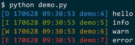
If logger.info(..) was called from a file called demo.py, the output will look like this:

example output with colors

[D 17062809:30:53 demo:4] hello
[I 17062809:30:53 demo:5] info
[W 17062809:30:53 demo:6] warn
[E 17062809:30:53 demo:7] error

You can also easily log to a file as well:

logger=setup_logger(logfile="/tmp/test.log")

This is how you can log variables too:

logger.debug("var1: %s, var2: %s",var1,var2)

This is how you can set the minimum logging level (default is DEBUG):

setup_logger(level=logging.INFO)

See also the documentation of setup_logger(..) for more details and options.


Installation

Install logzero with pip:

$ pip install -U logzero

If you don’t have pip installed, this Python installation guide can guide you through the process. Alternatively you can also install logzero from the Github repository with python setup.py install.


Take a look at the full documentation: https://logzero.readthedocs.io

If you have comments, feedback or suggestions, I’m happy to hear from you. Please reach out via @metachris!

Matthew Rocklin: Programmatic Bokeh Servers

$
0
0

This work is supported by Continuum Analytics

This was cross posted to the Bokeh blog here. Please consider referencing and sharing that post via social media instead of this one.

This blogpost shows how to start a very simple bokeh server application programmatically. For more complex examples, or for the more standard command line interface, see the Bokeh documentation.

Motivation

Many people know Bokeh as a tool for building web visualizations from languages like Python. However I find that Bokeh’s true value is in serving live-streaming, interactive visualizations that update with real-time data. I personally use Bokeh to serve real-time diagnostics for a distributed computing system. In this case I embed Bokeh directly into my library. I’ve found it incredibly useful and easy to deploy sophisticated and beautiful visualizations that help me understand the deep inner-workings of my system.

Most of the (excellent) documentation focuses on stand-alone applications using the Bokeh server

$ bokeh serve myapp.py

However as a developer who wants to integrate Bokeh into my application starting up a separate process from the command line doesn’t work for me. Also, I find that starting things from Python tends to be a bit simpler on my brain. I thought I’d provide some examples on how to do this within a Jupyter notebook.

Launch Bokeh Servers from a Notebook

The code below starts a Bokeh server running on port 5000 that provides a single route to / that serves a single figure with a line-plot. The imports are a bit wonky, but the amount of code necessary here is relatively small.

frombokeh.server.serverimportServerfrombokeh.applicationimportApplicationfrombokeh.application.handlers.functionimportFunctionHandlerfrombokeh.plottingimportfigure,ColumnDataSourcedefmake_document(doc):fig=figure(title='Line plot!',sizing_mode='scale_width')fig.line(x=[1,2,3],y=[1,4,9])doc.title="Hello, world!"doc.add_root(fig)apps={'/':Application(FunctionHandler(make_document))}server=Server(apps,port=5000)server.start()

We make a function make_document which is called every time someone visits our website. This function can create plots, call functions, and generally do whatever it wants. Here we make a simple line plot and register that plot with the document with the doc.add_root(...) method.

This starts a Tornado web server and creates a new image whenever someone connects, similar to libraries like Tornado, or Flask. In this case our web server piggybacks on the Jupyter notebook’s own IOLoop. Because Bokeh is built on Tornado it can play nicely with other async applications like Tornado or Asyncio.

Live Updates

I find that Bokeh’s real strength comes when you want to stream live data into the browser. Doing this by hand generally means serializing your data on the server, figuring out how web sockets work, sending the data to the client/browser and then updating plots in the browser.

Bokeh handles this by keeping a synchronized table of data on the client and the server, the ColumnDataSource. If you define plots around the column data source and then push more data into the source then Bokeh will handle the rest. Updating your plots in the browser just requires pushing more data into the column data source on the server.

In the example below every time someone connects to our server we make a new ColumnDataSource, make an update function that adds a new record into it, and set up a callback to call that function every 100ms. We then make a plot around that data source to render the data as colored circles.

Because this is a new Bokeh server we start this on a new port, though in practice if we had multiple pages we would just add them as multiple routes in the apps variable.

importrandomdefmake_document(doc):source=ColumnDataSource({'x':[],'y':[],'color':[]})defupdate():new={'x':[random.random()],'y':[random.random()],'color':[random.choice(['red','blue','green'])]}source.stream(new)doc.add_periodic_callback(update,100)fig=figure(title='Streaming Circle Plot!',sizing_mode='scale_width',x_range=[0,1],y_range=[0,1])fig.circle(source=source,x='x',y='y',color='color',size=10)doc.title="Now with live updating!"doc.add_root(fig)apps={'/':Application(FunctionHandler(make_document))}server=Server(apps,port=5001)server.start()

By changing around the figures (or combining multiple figures, text, other visual elements, and so on) you have full freedom over the visual styling of your web service. By changing around the update function you can pull data from sensors, shove in more interesting data, and so on. This toy example is meant to provide the skeleton of a simple application; hopefully you can fill in details from your application.

Real example

Here is a simple example taken from Dask’s dashboard that maintains a streaming time series plot with the number of idle and saturated workers in a Dask cluster.

defmake_document(doc):source=ColumnDataSource({'time':[time(),time()+1],'idle':[0,0.1],'saturated':[0,0.1]})x_range=DataRange1d(follow='end',follow_interval=20000,range_padding=0)fig=figure(title="Idle and Saturated Workers Over Time",x_axis_type='datetime',y_range=[-0.1,len(scheduler.workers)+0.1],height=150,tools='',x_range=x_range,**kwargs)fig.line(source=source,x='time',y='idle',color='red')fig.line(source=source,x='time',y='saturated',color='green')fig.yaxis.minor_tick_line_color=Nonefig.add_tools(ResetTool(reset_size=False),PanTool(dimensions="width"),WheelZoomTool(dimensions="width"))doc.add_root(fig)defupdate():result={'time':[time()*1000],'idle':[len(scheduler.idle)],'saturated':[len(scheduler.saturated)]}source.stream(result,10000)doc.add_periodic_callback(update,100)

You can also have buttons, sliders, widgets, and so on. I rarely use these personally though so they don’t interest me as much.

Final Thoughts

I’ve found the Bokeh server to be incredibly helpful in my work and also very approachable once you understand how to set one up (as you now do). I hope that this post serves people well. This blogpost is available as a Jupyter notebook if you want to try it out yourself.

Wesley Chun: Modifying events with the Google Calendar API

$
0
0
NOTE: The code featured here is also available as a video + overview post as part of this developers series from Google.

Introduction

In an earlier post, I introduced Python developers to adding events to users' calendars using the Google Calendar API. However, while being able to insert events is "interesting," it's only half the picture. If you want to give your users a more complete experience, modifying those events is a must-have. In this post, you'll learn how to modify existing events, and as a bonus, learn how to implement repeating events too.

In order to modify events, we need the full Calendar API scope:
  • 'https://www.googleapis.com/auth/calendar'—read-write access to Calendar
Skipping the OAuth2 boilerplate, once you have valid authorization credentials, create a service endpoint to the Calendar API like this:
GCAL = discovery.build('calendar', 'v3',
http=creds.authorize(Http()))
Now you can send the API requests using this endpoint.

Using the Google Calendar API

Our sample script requires an existing Google Calendar event, so either create one programmatically with events().insert()& save its ID as we showed you in that earlier post, or use events().list() or events().get() to get the ID of an existing event.

While you can use an offset from GMT/UTC, such as the GMT_OFF variable from the event insert post, today's code sample "upgrades" to a more general IANA timezone solution. For Pacific Time, it's "America/Los_Angeles". The reason for this change is to allow events that survive across Daylight Savings Time shifts. IOW, a dinner at 7PM/1900 stays at 7PM as we cross fall and spring boundaries. This is especially important for events that repeat throughout the year. Yes, we are discussing recurrence in this post too, so it's particularly relevant.

Modifying calendar events

In the other post, the EVENT body constitutes an "event record" containing the information necessary to create a calendar entry—it consists of the event name, start & end times, and invitees. That record is an API resource which you created/accessed with the Calendar API via events().insert(). (What do you think the "R" in "URL" stands for anyway?!?) The Calendar API adheres to RESTful semantics in that the HTTP verbs match the actions you perform against a resource.

In today's scenario, let's assume that dinner from the other post didn't work out, but that you want to reschedule it. Furthermore, not only do you want to make that dinner happen again, but because you're good friends, you've made a commitment to do dinner every other month for the rest of the year, then see where things stand. Now that we know what we want, we have a choice.

There are two ways to modifying existing events in Calendar:
  1. events().patch() (HTTP PATCH)—"patch" 1 or more fields in resource
  2. events().update() (HTTP PUT)—replace/rewrite entire resource
Do you just update that resource with events().patch() or do you replace the entire resource with events().update()? To answer that question, ask yourself, "How many fields am I updating?" In our case, we only want to change the date and make this event repeat, so PATCH is a better solution. If instead, you also wanted to rename the event or switch dinner to another set of friends, you'd then be changing all the fields, so PUT would be a better solution in that case.

Using PATCH means you're just providing the deltas between the original & updated event, so the EVENT body this time reflects just those changes:
TIMEZONE = 'America/Los_Angeles'
EVENT = {
'start': {'dateTime': '2017-07-01T19:00:00', 'timeZone': TIMEZONE},
'end': {'dateTime': '2017-07-01T22:00:00', 'timeZone': TIMEZONE},
'recurrence': ['RRULE:FREQ=MONTHLY;INTERVAL=2;UNTIL=20171231']
}

Repeating events

Something you haven't seen before is how to do repeating events. To do this, you need to define what’s known as a recurrence rule ("RRULE"), which answers the question of how often an event repeats. It looks somewhat cryptic but follows the RFC 5545 Internet standard which you can basically decode like this:
  • FREQ=MONTHLY—event to occur on a monthly basis...
  • INTERVAL=2—... but every two months (every other month)
  • UNTIL=20171231—... until this date
There are many ways events can repeat, so I suggest you look at all the examples at the RFC link above.

Finishing touches

Finally, provide the EVENT_ID and call events().patch():
EVENT_ID = YOUR_EVENT_ID_STR_HERE # use your own!
e = GCAL.events().patch(calendarId='primary', eventId=EVENT_ID,
sendNotifications=True, body=EVENT).execute()
Keep in mind that in real life, your users may be accessing your app from their desktop or mobile devices, so you need to ensure you don't override an earlier change. In this regard, developers should use the If-Match header along with an ETag value to validate unique requests. For more information, check out the conditional modification page in the official docs.

The one remaining thing is to confirm on-screen that the calendar event was updated successfully. We do that by checking the return value—it should be an Event object with all the existing details as well as the modified fields:
print('''\
*** %r event (ID: %s) modified:
Start: %s
End: %s
Recurring (rule): %s
''' % (e['summary'].encode('utf-8'), e['id'], e['start']['dateTime'],
e['end']['dateTime'], e['recurrence'][0]))
That's pretty much the entire script save for the OAuth2 boilerplate code we've explored previously. The script is posted below in its entirety, and if you add a valid event ID and run it, depending on the date/times you use, you'll see something like this:
$ python gcal_modify.py
*** 'Dinner with friends' event (ID: YOUR_EVENT_ID_STR_HERE) modified:
Start: 2017-07-01T19:00:00-07:00
End: 2017-07-01T22:00:00-07:00
Recurring (rule): RRULE:FREQ=MONTHLY;UNTIL=20171231;INTERVAL=2
It also works with Python 3 with one slight nit/difference being the "b" prefix on from the event name due to converting from Unicode to bytes:
*** b'Dinner with friends' event...

Conclusion

Now you know how to modify events as well as make them repeat. To complete the example, below is the entire script for your convenience which runs on both Python 2 and Python 3 (unmodified!):
from __future__ import print_function
from apiclient.discovery import build
from httplib2 import Http
from oauth2client import file, client, tools

SCOPES = 'https://www.googleapis.com/auth/calendar'
store = file.Storage('storage.json')
creds = store.get()
if not creds or creds.invalid:
flow = client.flow_from_clientsecrets('client_secret.json', SCOPES)
creds = tools.run_flow(flow, store)
CAL = build('calendar', 'v3', http=creds.authorize(Http()))

TIMEZONE = 'America/Los_Angeles'
EVENT = {
'start': {'dateTime': '2017-07-01T19:00:00', 'timeZone': TIMEZONE},
'end': {'dateTime': '2017-07-01T22:00:00', 'timeZone': TIMEZONE},
'recurrence': ['RRULE:FREQ=MONTHLY;INTERVAL=2;UNTIL=20171231']
}
EVENT_ID = YOUR_EVENT_ID_STR_HERE
e = GCAL.events().patch(calendarId='primary', eventId=EVENT_ID,
sendNotifications=True, body=EVENT).execute()

print('''\
*** %r event (ID: %s) modified:
Start: %s
End: %s
Recurring (rule): %s
''' % (e['summary'].encode('utf-8'), e['id'], e['start']['dateTime'],
e['end']['dateTime'], e['recurrence'][0]))
You can now customize this code for your own needs, for a mobile frontend, a server-side backend, or to access other Google APIs. If you want to learn more about using the Google Calendar API, check out the following resources:


Dataquest: Web Scraping with Python and BeautifulSoup

$
0
0

To source data for data science projects, you’ll often rely on SQL and NoSQL databases, APIs, or ready-made CSV data sets.

The problem is that you can’t always find a data set on your topic, databases are not kept current and APIs are either expensive or have usage limits.

If the data you’re looking for is on an web page, however, then the solution to all these problems is web scraping.

In this tutorial we’ll learn to scrape multiple web pages with Python using BeautifulSoup and requests. We’ll then perform some simple analysis using pandas, and matplotlib.

You should already have some basic understanding of HTML, a good grasp of Python’s basics, and a rough idea about what web scraping is. If you are not comfortable with these, I recommend this beginner web scraping tutorial.

Scraping data for over 2000 movies

We want to analyze the distributions of IMDB and Metacritic movie ratings to see if we find anything interesting. To do this, we’ll first scrape data for over 2000 movies.

It’s essential to identify...

Enthought: What’s New in the Canopy Data Import Tool Version 1.1

$
0
0

New features in the Canopy Data Import Tool Version 1.1:
Support for Pandas v. 20, Excel / CSV export capabilities, and more

Enthought Canopy Data Import ToolWe’re pleased to announce a significant new feature release of the Canopy Data Import Tool, version 1.1. The Data Import Tool allows users to quickly and easily import CSVs and other structured text files into Pandas DataFrames through a graphical interface, manipulate the data, and create reusable Python scripts to speed future data wrangling. Here are some of the notable updates in version 1.1:

1. Support for Python 3 and PyQt
The Data Import Tool now supports Python 3 and both PyQt and PySide backends.

2. Exporting DataFrames to csv/xlsx file formats
We understand that data exploration and manipulation are only one part of your data analysis process, which is why the Data Import Tool now provides a way for you to save the DataFrame as a CSV/XLSX file. This way, you can share processed data with your colleagues or feed this processed file to the next step in your data analysis pipeline.

3. Column Sort Indicators
In earlier versions of the Data Import Tool, it was not obvious that clicking on the right-end of the column header sorted the columns. With this release, we added sort indicators on every column, which can be pressed to sort the column in an ascending or descending fashion. And given the complex nature of the data we get, we know sorting the data based on single column is never enough, so we also made sorting columns using the Data Import Tool stable (ie, sorting preserves any existing order in the DataFrame).

4. Support for Pandas versions 0.19.2 – 0.20.1
Version 1.1 of the Data Import Tool now supports 0.19.2 and 0.20.1 versions of the Pandas library.

5. Column Name Selection
If duplicate column names exist in the data file, Pandas automatically mangles them to create unique column names. This mangling can be buggy at times, especially if there is whitespace around the column names. The Data Import Tool corrects this behavior to give a consistent user experience. Until the last release, this was being done under the hood by the Tool. With this release, we changed the Tool’s behavior to explicitly point out what columns are being renamed and how.

6. Template Discovery
With this release, we updated how a Template file is chosen for a given input file. If multiple template files are discovered to be relevant, we choose the latest. We also sped up loading data from files if a relevant Template is used.

For those of you new to the Data Import Tool, a Template file contains all of the commands you executed on the raw data using the Data Import Tool. A Template file is created when a DataFrame is successfully imported into the IPython console in the Canopy Editor. Further, a unique Template file is created for every data file.

Using Template files, you can save your progress and when you later reload the data file into the Tool, the Tool will automatically discover and load the right Template for you, letting you start off from where you left things.

7. Increased Cell Copy and Data Loading Speeds Copying cells has been sped up significantly. We also sped up loading data from large files (>70MB in size).


Using the Data Import Tool in Practice: a Machine Learning Use Case

In theory, we could look at the various machine learning models that can be used to solve our problems and jump right to training and testing the models.

However, in reality, a large amount of time is invested in the data cleaning and data preparation process. More often than not, real-life data cannot be simply fed to a machine learning model directly; there could be missing values, the data might need further processing to remove unnecessary details and join columns to generate a clean and concise dataset.

That’s where the Data Import Tool comes in. The Pandas library made the process of data cleaning and processing has gotten easier and now, the Data Import Tool makes it A LOT easier. By letting you visually clean your dataset, be it removing, converting or joining columns, the Data Import Tool will allow you to visually operate on the data frame and look at the outcome of the operations. Not only that, the Data Import Tool is stateful, meaning that every command can be reverted and changes can be undone.

To give you a real world example, let’s look at the training and test datasets from the Occupancy detection dataset. The dataset contains 8 columns of data, the first column contains index values, the second column contains DateTime values and the rest contain numerical values.

As soon as you try loading the dataset, you might get an error. This is because the dataset contains a row containing column headers for 7 columns. But, the rest of the dataset contains 8 columns of data, which includes the index column. Because of this, we will have to skip the first row of data, which can be done from the Edit Command pane of the ReadData command.

After we set `Number of rows to skip` to `1` and click `Refresh Data`, we should see the DataFrame we expect from the raw data. You might notice that the Data Import tool automatically converted the second column of data into a `DateTime` column. The DIT infers the type of data in a column and automatically performs the necessary conversions. Similarly, the last column was converted into a Boolean column because it represents the Occupancy, with values 0/1.

As we can see from the raw data, the first column in the data contains Index values.. We can access the `SetIndex` command from the right-click menu item on the `ID` column.

Alongside automatic conversions, the DIT generates the relevant Python/Pandas code, which can be saved from the `Save -> Save Code` sub menu item. The complete code generated when we loaded the training data set can be seen below:

# -*- coding: utf-8 -*-
import pandas as pd


# Pandas version check
from pkg_resources import parse_version
if parse_version(pd.__version__) != parse_version('0.19.2'):
raise RuntimeError('Invalid pandas version')


from catalyst.pandas.convert import to_bool, to_datetime
from catalyst.pandas.headers import get_stripped_columns

# Read Data from datatest.txt


filename = 'occupancy_data/datatest.txt'
data_frame = pd.read_table(
filename,
delimiter=',', encoding='utf-8', skiprows=1,
keep_default_na=False, na_values=['NA', 'N/A', 'nan', 'NaN', 'NULL', ''], comment=None,
header=None, thousands=None, skipinitialspace=True,
mangle_dupe_cols=True, quotechar='"',
index_col=False
)


# Ensure stripping of columns
data_frame = get_stripped_columns(data_frame)


# Type conversion for the following columns: 1, 7
for column in ['7']:
valid_bools = {0: False, 1: True, 'true': True, 'f': False, 't': True, 'false': False}
data_frame[column] = to_bool(data_frame[column], valid_bools)
for column in ['1']:
data_frame[column] = to_datetime(data_frame[column])

As you can see, the generated script shows how the training data can be loaded into a DataFrame using Pandas, how the relevant columns can be converted to Bool and DateTime type and how a column can be set as the Index of the DataFrame. We can trivially modify this script to perform the same operations on the other datasets by replacing the filename.

Finally, not only does the Data Import Tool generate and autosave a Python/Pandas script for each of the commands applied, it also saves them into a nifty Template file. The Template file aids in reproducibility and speeds up the analysis process.

Once you successfully modify the training data, every subsequent time you load the training data using the Data Import Tool, it will automatically apply the commands/operations you previously ran. Not only that, we know that the training and test datasets are similar and we need to perform the same data cleaning operations on both files.

Once we cleaned the training dataset using the Data Import Tool, if we load the test dataset, it will intelligently understand that we are loading a file similar to the training dataset and will automatically perform the same operations that we performed on the training data.

The datasets are available at – https://archive.ics.uci.edu/ml/datasets/Occupancy+Detection+#


Ready to try the Canopy Data Import Tool?

Download Canopy (free) and click on the icon to start a free trial of the Data Import Tool today.

(NOTE: The free trial is currently only available for Python 2.7 users. Python 3 users may request a free trial by emailing canopy.support@enthought.com. All paid Canopy subscribers have access to the Data Import Tool for both Python 2 and Python 3.)


We encourage you to update the latest version of the Data Import Tool in Canopy’s Package Manager (search for the “catalyst” package) to make the most of the updates.

For a complete list of changes, please refer to the Release Notes for the Version 1.1 of the Tool here. Refer to the Enthought Knowledge Base for Known Issues with the Tool.

Finally, if you would like to provide us feedback regarding the Data Import Tool, write to us at canopy.support@enthought.com.


Additional resources:

Related blogs:

Watch a 2-minute demo video to see how the Canopy Data Import Tool works:

See the Webinar “Fast Forward Through Data Analysis Dirty Work” for examples of how the Canopy Data Import Tool accelerates data munging:

The post What’s New in the Canopy Data Import Tool Version 1.1 appeared first on Enthought Blog.

Carl Chenet: Automatically Send Toots To The Mastodon Social Network

$
0
0

I’m a user of the new Twitter-like social network Mastodon and the need to automatize sending content on a regular basis to Mastodon soon pushed me to develop my own tools like Feed2toot (RSS to Mastodon) and Boost (automatically boost messages).

But I also needed a command-line client for the Mastodon Network in order to automatically toot on a regular basis.

Le réseau social Mastodon

After some time to compare the different available CLI clients, I fell in love with Toot, a command-line client for the Mastodon Network by Ivan Habunek. In the next chapters, I’ll explain how to install Toot and use it for simple message or more complex ones with images.

Install the Toot client

Just use Pip to install toot with the following command:

# pip3 install toot

Now you need to log in the instance you will send messages to with the following command:

$ toot login

If the credentials you provided are correct, you are now ready to toot! Let’s try to add the most simple possible toot on my timeline:

$ toot post test
Toot posted: https://mastodon.social/@carlchenet/11197113

Here is the result on my timeline:

Example of a toot sent from the command line

Adding line breaks in your toots

For a long time I could not use Toot for complex toots because I could not succeed adding line breaks in the message, which strongly restricts the possibilities.

Ivan Habunek, the creator of Toot, provided a solution replying to my bug report and I was soon using Toot like crazy! Here is how to add a line break in your toots:

$ toot post $'first line\n\nhow to escape a single quote \'\n\nlast line'

Here is the result:

How to use line breaks in your toots

Send toots with images

Ok, the last missing feature to send interesting toots for your followers is attaching images with your toots. With the Toot command line client, it’s quite easy. Just use the following command:

$ toot post -m /home/carlchenet/carlchenet-blog.png $'Read my blog for latest information about automatically sending content to #Mastodon\n\nMy Blog: https://carlchenet.com'

The option -m allows to attach an image. Every word starting with a # will be a hashtag and all urls will be correctly displayed. If you need to notify someone from the current instance, use the name of this account starting with a @. If his account is not on the same instance, use the full name @carlchenet@mastodon.social

Define when sending toots

Simple is beautiful, so I use my good old crontab. Considering my last example, I’ll create a simple script in /home/carlchenet/toot-advertise-carlchenet-blog.sh sending my toot:

#!/bin/bash
toot post -m /home/carlchenet/carlchenet-blog.png $'Read my blog for latest information about automatically sending content to #Mastodon\n\nMy Blog: https://carlchenet.com'
exit 0

Just make this script executable:

chmod u+x /home/carlchenet/toot-advertise-carlchenet-blog.sh

Last step to send my toot each day at 10AM, add a line in your crontab:

00 10 * * * carlchenet /home/carlchenet/toot-advertise-carlchenet-blog.sh

Now we’re ready! My toot will be sent to Mastodon every day at 10AM.

My Other blog Posts About Automatically Sending Content To Mastodon

With great powers come great responsabilities

The Toot client allows sending automatically really cool stuff to Mastodon, but always think about the noise for your users it can generate if you use it too much.

As always while automatizing stuff, use it in a smart way and everybody will enjoy it.

… and finally

You can help me developing tools for Mastodon by donating anything through Liberaypay (also possible with cryptocurrencies). Any contribution will be appreciated. That’s a big factor motivation 😉

You also may follow my account @carlchenet on Mastodon 😉

Carl Chenet On Mastodon

Stack Abuse: Python's @classmethod and @staticmethod Explained

$
0
0

Python is a unique language in that it is fairly easy to learn, given its straight-forward syntax, yet still extremely powerful. There are a lot more features under the hood than you might realize. While I could be referring to quite a few different things with this statement, in this case I'm talking about the decorators@classmethod and @staticmethod. For many of your projects, you probably didn't need or encounter these features, but you may find that they come in handy quite a bit more than you'd expect. It's not as obvious how to create Python static methods, which is where these two decorators come in.

In this article I'll be telling you what each of these decorators do, their differences, and some examples of each.

The @classmethod Decorator

This decorator exists so you can create class methods that are passed the actual class object within the function call, much like self is passed to any other ordinary instance method in a class.

In those instance methods, the self argument is the class instance object itself, which can then be used to act on instance data. @classmethod methods also have a mandatory first argument, but this argument isn't a class instance, it's actually the uninstantiated class itself. So, while a typical class method might look like this:

class Student(object):

    def __init__(self, first_name, last_name):
        self.first_name = first_name
        self.last_name = last_name

scott = Student('Scott',  'Robinson')  

A similar @classmethod method would be used like this instead:

class Student(object):

    @classmethod
    def from_string(cls, name_str):
        first_name, last_name = map(str, name_str.split(' '))
        student = cls(first_name, last_name)
        return student

scott = Student.from_string('Scott Robinson')  

This follows the static factory pattern very well, encapsulating the parsing logic inside of the method itself.

The above example is a very simple one, but you can imagine more complicated examples that make this more attractive. Imagine if a Student object could be serialized in to many different formats. You could use this same strategy to parse them all:

class Student(object):

    @classmethod
    def from_string(cls, name_str):
        first_name, last_name = map(str, name_str.split(' '))
        student = cls(first_name, last_name)
        return student

    @classmethod
    def from_json(cls, json_obj):
        # parse json...
        return student

    @classmethod
    def from_pickle(cls, pickle_file):
        # load pickle file...
        return student

The decorator becomes even more useful when you realize its usefulness in sub-classes. Since the class object is given to you within the method, you can still use the same @classmethod for sub-classes as well.

The @staticmethod Decorator

The @staticmethod decorator is similar to @classmethod in that it can be called from an uninstantiated class object, although in this case there is no cls parameter passed to its method. So an example might look like this:

class Student(object):

    @staticmethod
    def is_full_name(name_str):
        names = name_str.split(' ')
        return len(names) > 1

Student.is_full_name('Scott Robinson')   # True  
Student.is_full_name('Scott')            # False  

Since no self object is passed either, that means we also don't have access to any instance data, and thus this method can not be called on an instantiated object either.

These types of methods aren't typically meant to create/instantiate objects, but they may contain some type of logic pertaining to the class itself, like a helper or utility method.

@classmethod vs @staticmethod

The most obvious thing between these decorators is their ability to create static methods within a class. These types of methods can be called on uninstantiated class objects, much like classes using the static keyword in Java.

There is really only one difference between these two method decorators, but it's a major one. You probably noticed in the sections above that @classmethod methods have a cls parameter sent to their methods, while @staticmethod methods do not.

This cls parameter is the class object we talked about, which allows @classmethod methods to easily instantiate the class, regardless of any inheritance going on. The lack of this cls parameter in @staticmethod methods make them true static methods in the traditional sense. They're main purpose is to contain logic pertaining to the class, but that logic should not have any need for specific class instance data.

A Longer Example

Now let's see another example where we use both types together in the same class:

# static.py

class ClassGrades:

    def __init__(self, grades):
        self.grades = grades

    @classmethod
    def from_csv(cls, grade_csv_str):
        grades = map(int, grade_csv_str.split(', '))
        cls.validate(grades)
        return cls(grades)


    @staticmethod
    def validate(grades):
        for g in grades:
            if g < 0 or g > 100:
                raise Exception()

try:  
    # Try out some valid grades
    class_grades_valid = ClassGrades.from_csv('90, 80, 85, 94, 70')
    print 'Got grades:', class_grades_valid.grades

    # Should fail with invalid grades
    class_grades_invalid = ClassGrades.from_csv('92, -15, 99, 101, 77, 65, 100')
    print class_grades_invalid.grades
except:  
    print 'Invalid!'
$ python static.py
Got grades: [90, 80, 85, 94, 70]  
Invalid!  

Notice how the static methods can even work together with from_csv calling validate using the cls object. Running the code above should print out an array of valid grades, and then fail on the second attempt, thus printing out "Invalid!".

Conclusion

In this article you saw how both the @classmethod and @staticmethod decorators work in Python, some examples of each in action, and how they differ from each other. Hopefully now you can apply them to your own projects and use them to continue to improve the quality and organization of your own code.

Have you ever used these decorators before, and if so, how? Let us know in the comments!


Kushal Das: Second update from summer training 2017

$
0
0

We are already at the end of the second week of the dgplug summer training 2017. From this week onwards, we’ll have formal sessions only 3 days a week.
Guest lectures will start only from next month.
This post is a quick update about the things we did over the last 2 weeks.

  • Communication guideline review: We use Shakthi Kannan’s communication guideline and mailing list guideline in the training. We still have a few people having trouble with not typing SMS language in the chat or in the mailing list. But, we’re learning fast.
  • Basics of Linux command line tools: We used to have only the old logs and the TLDP bash guides for this. Last year I thought of writing a new book (along the lines of Python for you and me), but did not manage to push myself to do so. This year, I have started working on Linux command line for you and me, though I haven’t yet edited the things I’ve written yet. We are using this book as a starting point for the participants along with the old logs.
  • GNU Typist: We also ask people to practice typing. We suggest using gtypist to learn touch typing. There are a few blog posts from the participants talking about their experience.
  • We had two sessions on Vim. Sayan will take another special session on Vim in the coming days.
  • We talked about blogs, and asked everyone start writing more. Writing is important; be it technical documentation, or an email to a mailing list – it is the way to communicate over the Internet. We suggested Wordpress to the beginners. If you are interested to see what the participants are writing, visit the planet.
  • The Internet’s Own Boy: This week we also asked everyone to watch the story of Aaron Swartz. The summer training is not about just learning a few tools, or learning about projects. It is about people, about freedom. Freedom to do things, freedom to learn. One of our participants, Robin Schubert (who is a physicist from Germany) wrote his thoughts after watching the documentary. I am hoping that more participants will think more about what they saw.
    Following this, we will also have a session about the history of Free Software, and why we do, what we do. The ideology still matters. Without understanding or actually caring about the issues, just writing code will not help us in the future.
  • Next, we actually asked people to submit their RSS feeds so that we can add them to the planet. We also learned Markdown, and people noticed how Aaron was involved in the both.

In the coming days, we will learn about few more tools, and how to use programming to automate things in life. How to contribute patches to the upstream projects and such related things. But, we will also have sessions on software licenses. Anwesha will take the initial session on the same. The guest sessions will also start. If you are interested in teaching or sharing your story with the participants, please drop me a note (either email or twitter).

Brad Lucas: Coin Market Cap

$
0
0

There is a useful page called CryptoCurrency Market Capitalizations for viewing the current state of the crytocurency markets.

https://coinmarketcap.com/assets/views/all/

The site shows all currencies runing today on a number of platforms. I'm interested in the ones running on Ethereum which have a Market Cap. Since, the site doesn't have this specific filtering capability I thought it would make a good project to grab the data from the page and filter it the way I'd like.

To do this I decided to investigate Pandas and it's read_html function for pulling data in from html tables.

The following are notes for a Python script that I wrote to pull data from the CryptoCurrency Market Capitalizations, massage the data and show it in useful formats.

Requirements

Setup a virtualenv with the following libraries.

tabulate
pandas
beautifulsoup4
html5lib
lxml
numpy

Read Table

When you investigate the html returned for the page you need to find how the table of data is identified. On inspection you'll see that the table has an id of assets-all. The following shows how you can read this table with Pandas into a DataFrame.

url = 'https://coinmarketcap.com/assets/views/all/'

# Use Pandas to return first table on page
#
df = pd.read_html(url, attrs = {'id': 'assets-all'})[0]

Column Names

The columns have the names of the table columns which I think are a bit unwieldy to use because they have symols and spaces in them. I changed them to sorter single word names.

# Original column names
#
# [ 0,    1,         2,          3,          4,         5,                   6,            7,        8,     9
# ['#', 'Name', 'Platform', 'Market Cap', 'Price', 'Circulating Supply', 'Volume (24h)', '% 1h', '% 24h', '% 7d']

# New column names
#
df.columns = ['#', 'Name', 'Platform', 'MarketCap', 'Price', 'Supply', 'VolumeDay', 'pctHour', 'pctDay', 'pctWeek']

Data Cleanup

Looking at the data you'll see that number fields have $, % and comma characters. These need to be removed so we can sort them numerically. Also, all the columns have an object type and we'll need them to be some sort of numerica for proper behavior.

# Clean the data with 'numbers' by removing $, % and , characters
#
df['Price'] = df['Price'].str.replace('$', '')
df['MarketCap'] = df['MarketCap'].str.replace('$', '')
df['MarketCap'] = df['MarketCap'].str.replace(',', '')
df['VolumeDay'] = df['VolumeDay'].str.replace('$', '')
df['VolumeDay'] = df['VolumeDay'].str.replace(',', '')
df['VolumeDay'] = df['VolumeDay'].str.replace('Low Vol', '0')
df['pctHour'] = df['pctHour'].str.replace('%', '')
df['pctDay'] = df['pctDay'].str.replace('%', '')
df['pctWeek'] = df['pctWeek'].str.replace('%', '')

# Covert 'number' columns to numeric type so they will sort as we'd like
#
def coerce_df_columns_to_numeric(df, column_list):
    df[column_list] = df[column_list].apply(pd.to_numeric, errors='coerce')


coerce_df_columns_to_numeric(df, ['MarketCap', 'Price', 'Supply', 'VolumeDay', 'pctHour', 'pctDay', 'pctWeek'])

To have a column that sorts the name nicely you can create an upper case name.

# Build an upper case name column so we can sort on it more easily
#
df['NameUpper'] = map(lambda x: x.upper(), df['Name'])

And lastly, we only want the Ethereum data with rows which have a MarketCap value.

# Filter so we only have rows which are Ethereum and which have a value for Market Cap
#
df = df.loc[(df['Platform'] == 'Ethereum') & (df['MarketCap'] != '?')]

Report

The following is one report displayed using tabulate. The source code in the repo listed below shows a few other example reports. The following was generated at 2017-07-01 09:07.

Name                MarketCap     Price      Supply    VolumeDay
----------------  -----------  --------  ----------  -----------
Aragon               77232067       2.3    33605167       581475
Arcade Token          2605530       1.2     2164691            0
Augur               289609100     26.33    11000000      4210830
Basic Attenti...    140634000  0.140634  1000000000      1450090
BCAP                 17505300      1.75    10000000       123788
Bitpark Coin          5708738  0.076117    75000000            0
Chronobank           14923518     21.02      710113       541856
Cofound.it           22082125  0.176657   125000000       580521
Creditbit             8750042  0.736853    11874881       359370
DigixDAO            162637000     81.32     2000000       303509
Edgeless             44011846  0.538422    81742288       699753
Ethbits                  1306   0.00307      425388            0
Ethereum Movi...      3605906  0.540886     6666666         3786
Etheroll             28676126       4.1     7001623        25658
FirstBlood          128400869       1.5    85558371      8141070
Gnosis              357368003    323.53     1104590     12010600
Golem               384864116  0.462004   833032000      4593380
Humaniq              26695588  0.163919   162858414       349474
Iconomi             320927340      3.69    87000000      1517730
iDice                 1439145  0.916062     1571013         8511
iExec RLC            43572989  0.551063    79070793       210195
Legends Room          3330340      1.67     2000000       571581
Lunyr                 6812330      2.96     2297853       194785
Matchpool            18527325  0.247031    75000000       206184
MCAP                 98717644      4.84    20383236       265530
Melon                42662775     71.18      599400       318787
Minereum              3193667      5.29      603585        39461
Nexium               19845651  0.298334    66521586      1003330
Numeraire            66873477     54.66     1223451     11890600
Patientory           13120520  0.187436    70000000      1151120
Pluton               11699988     13.76      850000       129772
Quantum              23432939  0.284194    82454023       118966
Quantum Resis...     37007412  0.711681    52000000       546218
RouletteToken         5681468  0.562946    10092385        78663
Round                49461925   0.05819   850000000       304667
SingularDTV         100459800  0.167433   600000000       280495
Status              159849442   0.04606  3470483788     11907400
Swarm City           17365793      2.36     7357576        40417
TaaS                 21002345      2.58     8146001       194969
TokenCard            25058443      1.06    23644056       513609
Unity Ingot          16015247  0.079283   202000000       413868
Veritaseum          161739277     82.21     1967282       370198
VOISE                 1294737      1.57      825578         5121
vSlice               32649327  0.977803    33390496       175566
WeTrust              21296301  0.231111    92147500       251720
Wings                36238040  0.403954    89708333       425818
Xaurum               30743467  0.241862   127111604        74506
Yocoin                 720973  0.006826   105618830        87033

Ian Ozsvald: Kaggle’s Mercedes-Benz Greener Manufacturing

$
0
0

Kaggle are running a regression machine learning competition with Mercedes-Benz right now, it closes in a week and runs for about 6 weeks overall. I’ve managed to squeeze in 5 days to have a play (I managed about 10 days on the previous Quora competition). My goal this time was to focus on new tools that make it faster to get to ‘pretty good’ ML solutions. Specifically I wanted to play with:

Most of the 5 days were spent either learning the above tools or making some suggestions for YellowBrick, I didn’t get as far as creative feature engineering. Currently I’m in the top 50th percentile on the leaderboard using raw features, some dimensionality reduction and various estimators.

TPOT is rather interesting – it uses a genetic algorithm approach to evolve the hyperparameters of one or more (Stacked) estimators. One interesting outcome is that TPOT was presenting good models that I’d never have used – e.g. an AdaBoostRegressor & LassoLars or GradientBoostingRegressor & ElasticNet.

TPOT works with all sklearn-compatible classifiers including XGBoost (examples) but recently there’s been a bug with n_jobs and multiple processes. Due to this the current version had XGBoost disabled, it looks now like that bug has been fixed. As a result I didn’t get to use XGBoost inside TPOT, I did play with it separately but the stacked estimators from TPOT were superior. Getting up and running with TPOT took all of 30 minutes, after that I’d leave it to run overnight on my laptop. It definitely wants lots of CPU time. It is worth noting that auto-sklearn has a similar n_jobs bug and the issue is known in sklearn.

It does occur to me that almost all of the models developed by TPOT are subsequently discarded (you can get a list of configurations and scores). There’s almost certainly value to be had in building averaged models of combinations of these, I didn’t get to experiment with this.

Having developed several different stacks of estimators my final combination involved averaging these predictions with the trustable-model provided by another Kaggler. The mean of these three pushed me up to 0.55508. My only feature engineering involved various FeatureUnions with the FunctionTransformer based on dimensionality reduction.

YellowBrick was presented at our PyDataLondon 2017 conference (write-up) this year by Rebecca (we also did a book signing). I was able to make some suggestions for improvements on the RegressionPlot and PredictionError along with sharing some notes on visualising tree-based feature importances (along with noting a demo bug in sklearn). Having more visualisation tools can only help, I hope to develop some intuition about model failures from these sorts of diagrams.

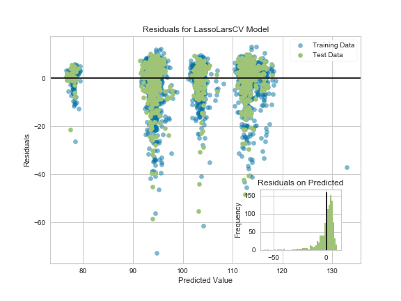
Here’s a ResidualPlot with my added inset prediction errors distribution, I think that this should be useful when comparing plots between classifiers to see how they’re failing:


Ian applies Data Science as an AI/Data Scientist for companies in ModelInsight, sign-up for Data Science tutorials in London. Historically Ian ran Mor Consulting. He also founded the image and text annotation API Annotate.io, co-authored SocialTies, programs Python, authored The Screencasting Handbook, lives in London and is a consumer of fine coffees.

Ian Ozsvald: PyDataLondon 2017 Conference write-up

$
0
0

Several weeks back we ran our 4th PyDataLondon (2017) conference– it was another smashing success! This builds on our previous 3 years of effort (2016, 2015, 2014) building both the conference and our over-subscribed monthly meetup. We’re grateful to our host Bloomberg for providing the lovely staff, venue and catering.

Really got inspired by @genekogan’s great talk on AI & the visual arts at @pydatalondon @annabellerol

Each year we try some new ideas – this year we tried:

pros: Great selection of talks for all levels and pub quiz cons: on a weekend, pub quiz (was hard). Overall would recommend 9/10 @harpal_sahota

We’re very thankful to all our sponsors for their financial support and to all our speakers for donating their time to share their knowledge. Personally I say a big thank-you to Ruby (co-chair) and Linda (review committee lead) – I resigned both of these roles this year after 3 years and I’m very happy to have been replaced so effectively (ahem – Linda – you really have shown how much better the review committee could be run!). Ruby joined Emlyn as co-chair for the conference, I took a back-seat on both roles and supported where I could. Our volunteer team great again – thanks Agata for pulling this together.

I believe we had 20% female attendees – up from 15% or so last year. Here’s a write-up from Srjdan and another from FullFact (and one from Vincent as chair at PyDataAmsterdam earlier this year) – thanks!

#PyDataLdn thank you for organising a great conference. My first one & hope to attend more. Will recommend it to my fellow humanists! @1208DL

For this year I’ve been collaborating with two colleagues – Dr Gusztav Belteki and Giles Weaver – to automate the analysis of baby ventilator data with the NHS. I was very happy to have the 3 of us present to speak on our progress, we’ve been using RandomForests to segment time-series breath data to (mostly) correctly identify the start of baby breaths on 100Hz single-channel air-flow data. This is the precursor step to starting our automated summarisation of a baby’s breathing quality.

Slides here and video below:

This updates our talk at the January PyDataLondon meetup. This collaboration came about after I heard of Dr. Belteki’s talk at PyConUK last year, whilst I was there to introduce RandomForests to Python engineers. You’re most welcome to come and join our monthly meetup if you’d like.

Many thanks to all of our sponsors again including Bloomberg for the excellent hosting and Continuum for backing the series from the start and NumFOCUS for bringing things together behind the scenes (and for supporting lots of open source projects – that’s where the money we raise goes to!).

There are plenty of other PyData and related conferences and meetups listed on the PyData website– if you’re interested in data then you really should get along. If you don’t yet contribute backto open source (and really – you should!) then do consider getting involved as a local volunteer. These events only work because of the volunteered effort of the core organising committees and extra hands (especially new members to the community) are very welcome indeed.

I’ll also note – if you’re in London or the south-east of the UK and you want to get a job in data science you should join my data scientist jobs email list, a set of companies who attended the conference have added their jobs for the next posting. Around 600 people are on this list and around 7 jobs are posted out every 2 weeks. Your email is always kept private.


Ian applies Data Science as an AI/Data Scientist for companies in ModelInsight, sign-up for Data Science tutorials in London. Historically Ian ran Mor Consulting. He also founded the image and text annotation API Annotate.io, co-authored SocialTies, programs Python, authored The Screencasting Handbook, lives in London and is a consumer of fine coffees.

Weekly Python Chat: Variables, scope, mutability

$
0
0

We're going to discuss the odd way that variables work in Python and how Python's variables differ from variables in other languages.

Viewing all 23144 articles
Browse latest View live


<script src="https://jsc.adskeeper.com/r/s/rssing.com.1596347.js" async> </script>