Quantcast
Channel: Planet Python
Viewing all 23369 articles
Browse latest View live

Experienced Django: KidsTasks – Working on Models

$
0
0

This is part two in the KidsTasks series where we’re designing and implementing a django app to manage daily task lists for my kids. See part 1 for details on requirements and goals.

Model Design Revisited

As I started coding up the models and the corresponding admin pages for the design I presented in the last section it became clear that there were several bad assumptions and mistakes in that design. (I plan to write up a post about designs and their mutability in the coming weeks.)

The biggest conceptual problem I had was the difference between “python objects” and “django models”. Django models correspond to database tables and thus do not map easily to things like “I want a list of Tasks in my DayOfWeekSchedule”.

After building up a subset of the models described in part 1, I found that the CountedTask model wasn’t going to work the way I had envisioned. Creating it as a direct subclass of Task caused unexpected (initially, at least) behavior in that all CountedTasks were also Tasks and thus showed up in all lists where Tasks could be added. While this behavior makes sense, it doesn’t fit the model I was working toward. After blundering with a couple of other ideas, it finally occurred to me that the main problem was the fundamental design. If something seems really cumbersome to implement it might be pointing to a design error.

Stepping back, it occurred to me that the idea of a “Counted” task was putting information at the wrong level. An individual task shouldn’t care if it’s one of many similar tasks in a Schedule, nor should it know how many there are. That information should be part of the Schedule models instead.

Changing this took more experimenting than I wanted, largely due to a mismatch in my thinking and how django models work. The key for working through this level of confusion was by trying to figure out how to add multiple Tasks of the same type to a Schedule. That led me to this Stack Overflow question which describes using an intermediate model to relate the two items. This does exactly what I’m looking for, allowing me to say that Kid1 needs to Practice Piano twice on Tuesdays without the need for a CountedTask model.

Changing this created problems for our current admin.py, however. I found ideas for how to clean that up here, which describes how to use inlines as part of the admin pages.

Using inlines and intermediate models, I was able to build up a schedule for a kid in a manner similar to my initial vision.  The next steps will be to work on views for this model and see where the design breaks!

Wrap Up

I’m going to stop this session here but I want to add a few interesting points and tidbits I’ve discovered on the way:

  • If you make big changes to the model and you don’t yet have any significant data, you can wipe out the database easily and start over with the following steps:
$rm db.sqlite3 tasks/migrations/ -rf$./manage.py makemigrations tasks$./manage.py migrate$./manage.py createsuperuser$./manage.py runserver
  • For models, it’s definitely worthwhile to add a __str__ (note: maybe __unicode__?) method and a Meta class to each one.  The __str__ method controls how the class is described, at least in the admin pages. The Meta class allows you to control the ordering when items of this model are listed. Cool!
  • I found (and forgot to note where) in the official docs an example of using a single char to store the name of the week while displaying the full day name. This looks like this:
    day_of_week_choices = (
        ('M', 'Monday'),
        ('T', 'Tuesday'),
        ('W', 'Wednesday'),
        ('R', 'Thursday'),
        ('F', 'Friday'),
        ('S', 'Saturday'),
        ('N', 'Sunday'),
    )
	...
    day_name = models.CharField(max_length=1, choices=day_of_week_choices)
  • NOTE that we’re going to have to tie the “name” fields in many of these models to the kid to which it’s associated. I’m considering if the kid can be combined into the schedule, but I don’t think that’s quite right. Certainly changes are coming to that part of the design.

That’s it! The state of the code at the point I’m writing this can be found here:

git@github.com:jima80525/KidTasks.git
git checkout blog/02-Models-first-steps

Thanks for reading!


Wesley Chun: Accessing Gmail from Python (plus BONUS)

$
0
0
NOTE: The code covered in this blogpost is also available in a video walkthrough here.

UPDATE (Aug 2016): The code has been modernized to use oauth2client.tools.run_flow() instead of the deprecated oauth2client.tools.run(). You can read more about that change here.

Introduction

The last several posts have illustrated how to connect to public/simple and authorized Google APIs. Today, we're going to demonstrate accessing the Gmail (another authorized) API. Yes, you read that correctly... "API." In the old days, you access mail services with standard Internet protocols such as IMAP/POP and SMTP. However, while they are standards, they haven't kept up with modern day email usage and developers' needs that go along with it. In comes the Gmail API which provides CRUD access to email threads and drafts along with messages, search queries, management of labels (like folders), and domain administration features that are an extra concern for enterprise developers.

Earlier posts demonstrate the structure and "how-to" use Google APIs in general, so the most recent posts, including this one, focus on solutions and apps, and use of specific APIs. Once you review the earlier material, you're ready to start with Gmail scopes then see how to use the API itself.

    Gmail API Scopes

    Below are the Gmail API scopes of authorization. We're listing them in most-to-least restrictive order because that's the order you should consider using them in  use the most restrictive scope you possibly can yet still allowing your app to do its work. This makes your app more secure and may prevent inadvertently going over any quotas, or accessing, destroying, or corrupting data. Also, users are less hesitant to install your app if it asks only for more restricted access to their inboxes.
    • 'https://www.googleapis.com/auth/gmail.readonly'— Read-only access to all resources + metadata
    • 'https://www.googleapis.com/auth/gmail.send' — Send messages only (no inbox read nor modify)
    • 'https://www.googleapis.com/auth/gmail.labels' — Create, read, update, and delete labels only
    • 'https://www.googleapis.com/auth/gmail.insert' — Insert and import messages only
    • 'https://www.googleapis.com/auth/gmail.compose'— Create, read, update, delete, and send email drafts and messages
    • 'https://www.googleapis.com/auth/gmail.modify'— All read/write operations except for immediate & permanent deletion of threads & messages
    • 'https://mail.google.com/'— All read/write operations (use with caution)

    Using the Gmail API

    We're going to create a sample Python script that goes through your Gmail threads and looks for those which have more than 2 messages, for example, if you're seeking particularly chatty threads on mailing lists you're subscribed to. Since we're only peeking at inbox content, the only scope we'll request is 'gmail.readonly', the most restrictive scope. The API string is 'gmail' which is currently on version 1, so here's the call to apiclient.discovery.build() you'll use:

    GMAIL = discovery.build('gmail', 'v1', http=creds.authorize(Http()))

    Note that all lines of code above that is predominantly boilerplate (that was explained in earlier posts). Anyway, once you have an established service endpoint with build(), you can use the list() method of the threads service to request the file data. The one required parameter is the user's Gmail address. A special value of 'me' has been set aside for the currently authenticated user.
    threads = GMAIL.users().threads().list(userId='me').execute().get('threads', [])
    If all goes well, the (JSON) response payload will (not be empty or missing and) contain a sequence of threads that we can loop over. For each thread, we need to fetch more info, so we issue a second API call for that. Specifically, we care about the number of messages in a thread:
    for thread in threads:
    tdata = GMAIL.users().threads().get(userId='me', id=thread['id']).execute()
    nmsgs = len(tdata['messages'])
    We're seeking only all threads more than 2 (that means at least 3) messages, discarding the rest. If a thread meets that criteria, scan the first message and cycle through the email headers looking for the "Subject" line to display to users, skipping the remaining headers as soon as we find one:
    if nmsgs > 2:
    msg = tdata['messages'][0]['payload']
    subject = ''
    for header in msg['headers']:
    if header['name'] == 'Subject':
    subject = header['value']
    break
    if subject:
    print('%s (%d msgs)' % (subject, nmsgs))
    If you're on many mailing lists, this may give you more messages than desired, so feel free to up the threshold from 2 to 50, 100, or whatever makes sense for you. (In that case, you should use a variable.) Regardless, that's pretty much the entire script save for the OAuth2 code that we're so familiar with from previous posts. The script is posted below in its entirety, and if you run it, you'll see an interesting collection of threads... YMMV depending on what messages are in your inbox:
    $ python3 gmail_threads.py
    [Tutor] About Python Module to Process Bytes (3 msgs)
    Core Python book review update (30 msgs)
    [Tutor] scratching my head (16 msgs)
    [Tutor] for loop for long numbers (10 msgs)
    [Tutor] How to show the listbox from sqlite and make it searchable? (4 msgs)
    [Tutor] find pickle and retrieve saved data (3 msgs)

    BONUS: Python 3!

    As of Mar 2015 (formally in Apr 2015 when the docs were updated), support for Python 3 was added to Google APIs Client Library (3.3+)! This update was a long time coming (relevant GitHub thread), and allows Python 3 developers to write code that accesses Google APIs. If you're already running 3.x, you can use its pip command (pip3) to install the Client Library:

    $ pip3 install -U google-api-python-client

    Because of this, unlike previous blogposts, we're deliberately going to avoid use of the print statement and switch to the print() function instead. If you're still running Python 2, be sure to add the following import so that the code will also run in your 2.x interpreter:

    from __future__ import print_function

    Conclusion

    To find out more about the input parameters as well as all the fields that are in the response, take a look at the docs for threads().list(). For more information on what other operations you can execute with the Gmail API, take a look at the reference docs and check out the companion video for this code sample. That's it!

    Below is the entire script for your convenience which runs on both Python 2 and Python 3 (unmodified!):
    from __future__ import print_function

    from apiclient import discovery
    from httplib2 import Http
    from oauth2client import file, client, tools

    SCOPES = 'https://www.googleapis.com/auth/gmail.readonly'
    store = file.Storage('storage.json')
    creds = store.get()
    if not creds or creds.invalid:
    flow = client.flow_from_clientsecrets('client_secret.json', SCOPES)
    creds = tools.run_flow(flow, store)
    GMAIL = discovery.build('gmail', 'v1', http=creds.authorize(Http()))

    threads = GMAIL.users().threads().list(userId='me').execute().get('threads', [])
    for thread in threads:
    tdata = GMAIL.users().threads().get(userId='me', id=thread['id']).execute()
    nmsgs = len(tdata['messages'])

    if nmsgs > 2:
    msg = tdata['messages'][0]['payload']
    subject = ''
    for header in msg['headers']:
    if header['name'] == 'Subject':
    subject = header['value']
    break
    if subject:
    print('%s (%d msgs)' % (subject, nmsgs))

    You can now customize this code for your own needs, for a mobile frontend, a server-side backend, or to access other Google APIs. If you want to see another example of using the Gmail API (displaying all your inbox labels), check out the Python Quickstart example in the official docs or its equivalent in Java (server-side, Android), iOS (Objective-C, Swift), C#/.NET, PHP, Ruby, JavaScript (client-side, Node.js), or Go. That's it... hope you find these code samples useful in helping you get started with the Gmail API!

    EXTRA CREDIT: To test your skills and challenge yourself, try writing code that allows users to perform a search across their email, or perhaps creating an email draft, adding attachments, then sending them! Note that to prevent spam, there are strict Program Policies that you must abide with... any abuse could rate limit your account or get it shut down. Check out those rules plus other Gmail terms of use here.

    Python Piedmont Triad User Group: PYPTUG Monthly meeting September 27th 2016 (Just bring Glue)

    $
    0
    0

    Come join PYPTUG at out next monthly meeting (August 30th 2016) to learn more about the Python programming language, modules and tools. Python is the perfect language to learn if you've never programmed before, and at the other end, it is also the perfect tool that no expert would do without. Monthly meetings are in addition to our project nights.


    What

    Meeting will start at 6:00pm.

    We will open on an Intro to PYPTUG and on how to get started with Python, PYPTUG activities and members projects, in particular some updates on the Quadcopter project, then on to News from the community.

    Then on to the main talk. If you missed Rob Agle's talk at PyData Carolinas (http://pydata.org/carolinas2016/schedule/presentation/62/), here is your chance. This will be an extended version.

     
    Main Talk: Just Bring Glue - Leveraging Multiple Libraries To Quickly Build Powerful New Tools
    by Rob Agle
    Bio:
    Rob Agle is a software engineer at Inmar, where he works on the high-availability REST APIs powering the organization's digital promotions network. His technical interests include application and network security, machine learning and natural language processing.

    Abstract:
    It has never been easier for developers to create simple-yet-powerful data-driven or data-informed tools. Through case studies, we'll explore a few projects that use a number of open source libraries or modules in concert. Next, we'll cover strategies for learning these new tools. Finally, we wrap up with pitfalls to keep in mind when gluing powerful things together quickly.

    Lightning talks! 


    We will have some time for extemporaneous "lightning talks" of 5-10 minute duration. If you'd like to do one, some suggestions of talks were provided here, if you are looking for inspiration. Or talk about a project you are working on.


    When

    Tuesday, September 27th 2016
    Meeting starts at 6:00PM

    Where

    Wake Forest University, close to Polo Rd and University Parkway:

    Wake Forest University, Winston-Salem, NC 27109


    And speaking of parking:  Parking after 5pm is on a first-come, first-serve basis.  The official parking policy is:
    "Visitors can park in any general parking lot on campus. Visitors should avoid reserved spaces, faculty/staff lots, fire lanes or other restricted area on campus. Frequent visitors should contact Parking and Transportation to register for a parking permit."

    Mailing List


    Don't forget to sign up to our user group mailing list:


    It is the only step required to become a PYPTUG member.

    RSVP on meetup:
    https://www.meetup.com/PYthon-Piedmont-Triad-User-Group-PYPTUG/events/233759543/

    Andre Roberge: Backward incompatible change in handling permalinks with Reeborg coming soon

    $
    0
    0
    About two years ago, I implemented a permalink scheme which was intended to facilitate sharing various programming tasks in Reeborg's World. As I added new capabilities, the number of possible items to include grew tremendously. In fact, for rich enough worlds, the permalink can be too long for the browser to handle. To deal with such situations, I had to implement a clumsy way to import and

    Curtis Miller: An Introduction to Stock Market Data Analysis with Python (Part 1)

    S. Lott: What was I thinking?

    $
    0
    0
    Check out this idiocy: https://github.com/slott56/py-false

    What is the point? Seriously. What. The. Actual. Heck?

    I think of it this way.

    • Languages are a cool thing. Especially programming languages where there's an absolute test -- the Turing machine -- for completeness. 
    • The Forth-like stack language is a cool thing. I've always liked Forth because if it's elegant simplicity. 
    • The use of a first-class lambda construct to implement if and while is particularly elegant.
    • Small languages are fun because they can be understood completely. There are no tricky edge cases in the semantics.
    I have ½ of a working GW-Basic implementation in Python, too. It runs. It runs some programs like HamCalc sort of okay-ish. I use it to validate assumptions about the legacy code in https://github.com/slott56/HamCalc-2.1.  Some day, I may make a sincere effort to get it working.

    Even languages like the one that supports the classic Adventure game are part of this small language fascination. See adventure.pdf for a detailed analysis of this game; this includes the little language you use to interact with the game.

    Tim Golden: Rambling Thoughts on PyCon UK 2016

    $
    0
    0

    If you track back through my write-ups of my previous PyCon UK experiences, you’ll see a bit of a trend: every year I say something like “This year was different”. And so it was this year. But this year it was differently different: it was different for the whole of PyCon UK, not just for me.

    PyCon UK was famously the brainchild of John Pinner (RIP) and was organised and run by him and a team of Python enthusiasts from the West Midlands with help from elsewhere. But we had clearly outgrown our Coventry venue: in the last two or three years, the facilities have become increasingly strained.

    So this year we were in Cardiff where Daniele Procida and others have successfully organised DjangoCon several times. Specifically we were in the City Hall which gave the conference more capacity and, I’m told, a slightly more responsive building staff over the weekend. I haven’t seen many facts or figures from the organisers, but certainly over 500 people were registered, in contrast to something like 300 for the last couple of years in Coventry. I don’t know if that’s because the size of the venue allowed more tickets to be made available or because Python has had a popularity explosion in the UK. I also don’t know whether it includes the Teachers’ and Children’s tickets, or those for the Open Day. Still: bigger.

    I was unable to take any time off work around the conference. We have a highly important deadline fast approaching for a Big Contract and all shore leave was cancelled. I was especially sorry to miss the Education Day for teachers, which I’ve been involved with since its inception 4 or 5 years ago. So when I finally arrived on Saturday morning, I went straight into the Kids’ track which was running a Code Club session on Racing Turtles. I’d heard not long before the Conference that there hadn’t been much take up for the Kids’ Day, so I was very glad to see that the place was packed with children & their parents. Unscientifically, I’d say that most were between 9-12 with a small number above and below those ages. Probably rather more girls than boys.

    After the break, there were sessions on Minecraft and micro:bit. I helped with the latter – I’m not a fan of Minecraft! And after lunch was a free-for-all in the Kids’ Track. The idea was to work on anything which had taken your fancy in the morning. I know from previous years that this sometimes works and sometimes doesn’t. (Generally parents of younger kids who are disengaged tend to take them away at this point). But for those old enough, or whose parents are keen enough, it was a great chance to explore possibilities. At different times there were quite a few conference-goers popping and out to offer help, although sometimes it’s not needed as everyone has their head down in a project.

    I always enjoy the youngsters at Python. Of course, not every child gets as much out of things as they might do. Some of the worksheets needed a lot of reading and then a lot of typing which was daunting especially to some younger participants. (And laziness is A Thing, of course!). But it’s great when the children get the bit between their teeth and get excited about what they’ve achieved… and that they worked it out themselves, and debugged it themselves. And they’ve got an idea about where to go next.

    For various reasons I spent relatively little time at the Conference proper. In particular, I only attended three talks, all of them given by people I knew and containing few surprises. It’s nice to see that several projects which I was slightly connected with early on have grown considerably and definitely merit a newer look: GPIOZero, PyGame Zero and PiNet. Like everyone else, I was impressed by the talk transcribers.The Conference venue was very pleasant and what I saw of Cardiff was welcoming – even though they were milking their connection with Roald Dahl, who’d been born there 100 years before.

    People have spoken and tweeted about how welcoming and open PyCon UK was for them, and I’m delighted. For me, the experience was a mixed one, I think for two reasons. One was that I was there for considerably less than 48 hours: I arrived on Saturday morning and left mid-afternoon on Sunday. I had necessarily little time to interact with people and, once I’d helped with the Kids’ Track, I particularly wanted to catch up with Andrew Mulholland of PiNet fame, and to say hello to people I pretty much only see at PyCon UK. Floris wanted to chat about networkzero and, once I’d done all that, it was almost time to go. I had an hour in the glorious Quiet Room (aka Cardiff City Council Chamber) before heading off on a coach to Bristol followed by a 2+hr stand on the train back to London.

    The other thing which muted my experience was how much bigger the Conference was this year, how many more people. Obviously, the fact of its being in South Wales will have skewed the catchment area, so to speak. But I was surprised at how few people I knew. Of course, at one level, this is great: the Python community is big and getting bigger; I’m not in an echo chamber where I talk to the same 12 people every year; people from the South & West who couldn’t get to Coventry can get to Cardiff. At the same time, I was irrationally lower in spirits (partly through lack of sleep, no doubt!). Normally I have no difficulty in just stopping by people to say things like “My name’s Tim; what do you use Python for?”. But this year, I just found it harder. So – sorry to people whom I appeared to be ignoring or who found me distracted.

    In particular I realised how much I’d missed by not being there the previous two days: it’s a little like starting at a new school when everyone else has already been there a while. There’s nothing I could have done, but I regretted it nonetheless. Hopefully it’ll be better next year.

    I look forward to seeing other people’s post-Conference write-ups and photos. I’m especially interested in people who didn’t enjoy things, or at least weren’t bowled over. Not because I’m reaching out for negativity, but because surely some people will have had an indifferent or even a negative experience at some level, and it would be good to understand why.

    Well there’s more I could say, but if you’ve even read this far, that’s more than I expected. I hope I’ll see you there next year, and meanwhile enjoy the tweets.

    Real Python: Caching in Django with Redis

    $
    0
    0
    django redis cache

    Application performance is vital to the success of your product. In an environment where users expect website response times of less than a second, the consequences of a slow application can be measured in dollars and cents. Even if you are not selling anything, fast page loads improve the experience of visiting your site.

    Everything that happens on the server between the moment it receives a request to the moment it returns a response increases the amount of time it takes to load a page. As a general rule of thumb, the more processing you can eliminate on the server, the faster your application will perform. Caching data after it has been processed and then serving it from the cache the next time it is requested is one way to relieve stress on the server. In this tutorial, we will explore some of the factors that bog down your application, and we will demonstrate how to implement caching with Redis to counteract their effects.

    What is Redis?

    Redis is an in-memory data structure store that can be used as a caching engine. Since it keeps data in RAM, Redis can deliver it very quickly. Redis is not the only product that we can use for caching. Memcached is another popular in-memory caching system, but many people agree that Redis is superior to Memcached in most circumstances. Personally, we like how easy it is to set up and use Redis for other purposes such as Redis Queue.

    Getting Started

    We have created an example application to introduce you to the concept of caching. Our application uses:

    Install the App

    Before you clone the repository, install virtualenvwrapper, if you don’t already have it. This is a tool that lets you install the specific Python dependencies that your project needs, allowing you to target the versions and libraries required by your app in isolation.

    Next, change directories to where you keep projects and clone the example app repository. Once done, change directories to the cloned repository, and then make a new virtual environment for the example app using the mkvirtualenv command:

    12
    $ mkvirtualenv django-redis
    (django-redis)$

    NOTE: Creating a virtual environment with mkvirtualenv also activates it.

    Install all of the required Python dependencies with pip, and then checkout the following tag:

    1
    (django-redis)$ git checkout tags/1
    

    Finish setting up the example app by building the database and populating it with sample data. Make sure to create a superuser too, so that you can log into the admin site. Follow the code examples below and then try running the app to make sure it is working correctly. Visit the admin page in the browser to confirm that the data has been properly loaded.

    1234
    (django-redis)$ python manage.py migrate
    (django-redis)$ python manage.py createsuperuser
    (django-redis)$ python manage.py loaddata cookbook/fixtures/cookbook.json
    (django-redis)$ python manage.py runserver
    

    Once you have the Django app running, move onto the Redis installation.

    Install Redis

    Download and install Redis using the instructions provided in the documentation. Alternatively, you can install Redis using a package manager such as apt-get or homebrew depending on your OS.

    Run the Redis server from a new terminal window.

    1
    $ redis-server
    

    Next, start up the Redis command-line interface (CLI) in a different terminal window and test that it connects to the Redis server. We will be using the Redis CLI to inspect the keys that we add to the cache.

    12
    $ redis-cli ping
    PONG
    

    Redis provides an API with various commands that a developer can use to act on the data store. Django uses django-redis to execute commands in Redis.

    Looking at our example app in a text editor, we can see the Redis configuration in the settings.py file. We define a default cache with the CACHES setting, using a built-in django-redis cache as our backend. Redis runs on port 6379 by default, and we point to that location in our setting. One last thing to mention is that django-redis appends key names with a prefix and a version to help distinguish similar keys. In this case, we have defined the prefix to be “example”.

    12345678910
    CACHES={"default":{"BACKEND":"django_redis.cache.RedisCache","LOCATION":"redis://127.0.0.1:6379/1","OPTIONS":{"CLIENT_CLASS":"django_redis.client.DefaultClient"},"KEY_PREFIX":"example"}}

    NOTE: Although we have configured the cache backend, none of the view functions have implemented caching.

    App Performance

    As we mentioned at the beginning of this tutorial, everything that the server does to process a request slows the application load time. The processing overhead of running business logic and rendering templates can be significant. Network latency affects the time it takes to query a database. These factors come into play every time a client sends an HTTP request to the server. When users are initiating many requests per second, the effects on performance become noticeable as the server works to process them all.

    When we implement caching, we let the server process a request once and then we store it in our cache. As requests for the same URL are received by our application, the server pulls the results from the cache instead of processing them anew each time. Typically, we set a time to live on the cached results, so that the data can be periodically refreshed, which is an important step to implement in order to avoid serving stale data.

    You should consider caching the result of a request when the following cases are true:

    • rendering the page involves a lot of database queries and/or business logic,
    • the page is visited frequently by your users,
    • the data is the same for every user,
    • and the data does not change often.

    Start by Measuring Performance

    Begin by testing the speed of each page in your application by benchmarking how quickly your application returns a response after receiving a request.

    To achieve this, we’ll be blasting each page with a burst of requests using loadtest, an HTTP load generator, and then paying close attention to the request rate. Visit the link above to install. Once installed, test the results against the /cookbook/ URL path:

    1
    $ loadtest -n 100 -k  http://localhost:8000/cookbook/
    

    Notice that we are processing about 16 requests per second:

    1
    Requests per second: 16
    

    When we look at what the code is doing, we can make decisions on how to make changes to improve the performance. The application makes 3 network calls to a database with each request to /cookbook/, and it takes time for each call to open a connection and execute a query. Visit the /cookbook/ URL in your browser and expand the Django Debug Toolbar tab to confirm this behavior. Find the menu labeled “SQL” and read the number of queries:

    django debug framework sql queries

    cookbook/services.py

    1234567
    fromcookbook.modelsimportRecipedefget_recipes():# Queries 3 tables: cookbook_recipe, cookbook_ingredient,# and cookbook_food.returnlist(Recipe.objects.prefetch_related('ingredient_set__food'))

    cookbook/views.py

    12345678
    fromdjango.shortcutsimportrenderfromcookbook.servicesimportget_recipesdefrecipes_view(request):returnrender(request,'cookbook/recipes.html',{'recipes':get_recipes()})

    The application also renders a template with some potentially expensive logic.

    12345678910111213141516171819
    <html><head><title>Recipes</title></head><body>{% for recipe in recipes %}
    <h1>{{ recipe.name }}</h1><p>{{ recipe.desc }}</p><h2>Ingredients</h2><ul>    {% for ingredient in recipe.ingredient_set.all %}
    <li>{{ ingredient.desc }}</li>    {% endfor %}
    </ul><h2>Instructions</h2><p>{{ recipe.instructions }}</p>{% endfor %}
    </body></html>

    Implement Caching

    Imagine the total number of network calls that our application will make as users start to visit our site. If 1,000 users hit the API that retrieves cookbook recipes, then our application will query the database 3,000 times and a new template will be rendered with each request. That number only grows as our application scales. Luckily, this view is a great candidate for caching. The recipes in a cookbook rarely change, if ever. Also, since viewing cookbooks is the central theme of the app, the API retrieving the recipes is guaranteed to be called frequently.

    In the example below, we modify the view function to use caching. When the function runs, it checks if the view key is in the cache. If the key exists, then the app retrieves the data from the cache and returns it. If not, Django queries the database and then stashes the result in the cache with the view key. The first time this function is run, Django will query the database and render the template, and then will also make a network call to Redis to store the data in the cache. Each subsequent call to the function will completely bypass the database and business logic and will query the Redis cache.

    example/settings.py

    12
    # Cache time to live is 15 minutes.CACHE_TTL=60*15

    cookbook/views.py

    1234567891011121314
    fromdjango.confimportsettingsfromdjango.core.cache.backends.baseimportDEFAULT_TIMEOUTfromdjango.shortcutsimportrenderfromdjango.views.decorators.cacheimportcache_pagefromcookbook.servicesimportget_recipesCACHE_TTL=getattr(settings,'CACHE_TTL',DEFAULT_TIMEOUT)@cache_page(CACHE_TTL)defrecipes_view(request):returnrender(request,'cookbook/recipes.html',{'recipes':get_recipes()})

    Notice that we have added the @cache_page() decorator to the view function, along with a time to live. Visit the /cookbook/ URL again and examine the Django Debug Toolbar. We see that 3 database queries are made and 3 calls are made to the cache in order to check for the key and then to save it. Django saves two keys (1 key for the header and 1 key for the rendered page content). Reload the page and observe how the page activity changes. The second time around, 0 calls are made to the database and 2 calls are made to the cache. Our page is now being served from the cache!

    When we re-run our performance tests, we see that our application is loading faster.

    1
    $ loadtest -n 100 -k  http://localhost:8000/cookbook/
    

    Caching improved the total load, and we are now resolving 21 requests per second, which is 5 more than our baseline:

    1
    Requests per second: 21
    

    Inspecting Redis with the CLI

    At this point we can use the Redis CLI to look at what gets stored on the Redis server. In the Redis command-line, enter the keys * command, which returns all keys matching any pattern. You should see a key called “example:1:views.decorators.cache.cache_page”. Remember, “example” is our key prefix, “1” is the version, and “views.decorators.cache.cache_page” is the name that Django gives the key. Copy the key name and enter it with the get command. You should see the rendered HTML string.

    12345
    $ redis-cli -n 1
    127.0.0.1:6379[1]> keys *
    1)"example:1:views.decorators.cache.cache_header"2)"example:1:views.decorators.cache.cache_page"127.0.0.1:6379[1]> get "example:1:views.decorators.cache.cache_page"

    NOTE: Run the flushall command on the Redis CLI to clear all of the keys from the data store. Then, you can run through the steps in this tutorial again without having to wait for the cache to expire.

    Wrap-up

    Processing HTTP requests is costly, and that cost adds up as your application grows in popularity. In some instances, you can greatly reduce the amount of processing your server does by implementing caching. This tutorial touched on the basics of caching in Django with Redis, but it only skimmed the surface of a complex topic. Implementing caching in a robust application has many pitfalls and gotchas. Controlling what gets cached and for how long is tough. Cache invalidation is one of the hard things in Computer Science. Ensuring that private data can only be accessed by its intended users is a security issue and must be handled very carefully when caching. Play around with the source code in the example application and as you continue to develop with Django, remember to always keep performance in mind.


    Ruslan Spivak: Let’s Build A Simple Interpreter. Part 11.

    $
    0
    0

    I was sitting in my room the other day and thinking about how much we had covered, and I thought I would recap what we’ve learned so far and what lies ahead of us.

    Up until now we’ve learned:

    • How to break sentences into tokens. The process is called lexical analysis and the part of the interpreter that does it is called a lexical analyzer, lexer, scanner, or tokenizer. We’ve learned how to write our own lexer from the ground up without using regular expressions or any other tools like Lex.
    • How to recognize a phrase in the stream of tokens. The process of recognizing a phrase in the stream of tokens or, to put it differently, the process of finding structure in the stream of tokens is called parsing or syntax analysis. The part of an interpreter or compiler that performs that job is called a parser or syntax analyzer.
    • How to represent a programming language’s syntax rules with syntax diagrams, which are a graphical representation of a programming language’s syntax rules. Syntax diagrams visually show us which statements are allowed in our programming language and which are not.
    • How to use another widely used notation for specifying the syntax of a programming language. It’s called context-free grammars (grammars, for short) or BNF (Backus-Naur Form).
    • How to map a grammar to code and how to write a recursive-descent parser.
    • How to write a really basic interpreter.
    • How associativity and precedence of operators work and how to construct a grammar using a precedence table.
    • How to build an Abstract Syntax Tree (AST) of a parsed sentence and how to represent the whole source program in Pascal as one big AST.
    • How to walk an AST and how to implement our interpreter as an AST node visitor.

    With all that knowledge and experience under our belt, we’ve built an interpreter that can scan, parse, and build an AST and interpret, by walking the AST, our very first complete Pascal program. Ladies and gentlemen, I honestly think if you’ve reached this far, you deserve a pat on the back. But don’t let it go to your head. Keep going. Even though we’ve covered a lot of ground, there are even more exciting parts coming our way.

    With everything we’ve covered so far, we are almost ready to tackle topics like:

    • Nested procedures and functions
    • Procedure and function calls
    • Semantic analysis (type checking, making sure variables are declared before they are used, and basically checking if a program makes sense)
    • Control flow elements (like IF statements)
    • Aggregate data types (Records)
    • More built-in types
    • Source-level debugger
    • Miscellanea (All the other goodness not mentioned above :)

    But before we cover those topics, we need to build a solid foundation and infrastructure.

    This is where we start diving deeper into the super important topic of symbols, symbol tables, and scopes. The topic itself will span several articles. It’s that important and you’ll see why. Okay, let’s start building that foundation and infrastructure, then, shall we?

    First, let’s talk about symbols and why we need to track them. What is a symbol? For our purposes, we’ll informally define symbol as an identifier of some program entity like a variable, subroutine, or built-in type. For symbols to be useful they need to have at least the following information about the program entities they identify:

    • Name (for example, ‘x’, ‘y’, ‘number’)
    • Category (Is it a variable, subroutine, or built-in type?)
    • Type (INTEGER, REAL)

    Today we’ll tackle variable symbols and built-in type symbols because we’ve already used variables and types before. By the way, the “built-in” type just means a type that hasn’t been defined by you and is available for you right out of the box, like INTEGER and REAL types that you’ve seen and used before.

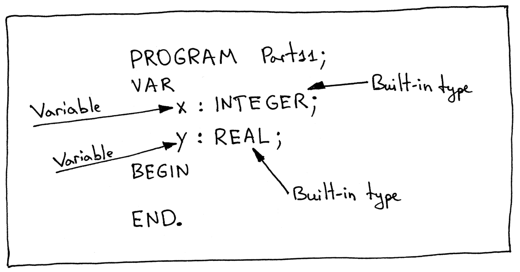
    Let’s take a look at the following Pascal program, specifically at the variable declaration part. You can see in the picture below that there are four symbols in that section: two variable symbols (x and y) and two built-in type symbols (INTEGER and REAL).

    How can we represent symbols in code? Let’s create a base Symbol class in Python:

    classSymbol(object):def__init__(self,name,type=None):self.name=nameself.type=type

    As you can see, the class takes the name parameter and an optional type parameter (not all symbols may have a type associated with them). What about the category of a symbol? We’ll encode the category of a symbol in the class name itself, which means we’ll create separate classes to represent different symbol categories.

    Let’s start with basic built-in types. We’ve seen two built-in types so far, when we declared variables: INTEGER and REAL. How do we represent a built-in type symbol in code? Here is one option:

    classBuiltinTypeSymbol(Symbol):def__init__(self,name):super(BuiltinTypeSymbol,self).__init__(name)def__str__(self):returnself.name__repr__=__str__

    The class inherits from the Symbol class and the constructor requires only a name of the type. The category is encoded in the class name, and the type parameter from the base class for a built-in type symbol is None. The double underscore or dunder (as in “Double UNDERscore”) methods __str__ and __repr__ are special Python methods and we’ve defined them to have a nice formatted message when you print a symbol object.

    Download the interpreter file and save it as spi.py; launch a python shell from the same directory where you saved the spi.py file, and play with the class we’ve just defined interactively:

    $ python
    >>> from spi import BuiltinTypeSymbol
    >>> int_type= BuiltinTypeSymbol('INTEGER')>>> int_type
    INTEGER
    >>> real_type= BuiltinTypeSymbol('REAL')>>> real_type
    REAL
    

    How can we represent a variable symbol? Let’s create a VarSymbol class:

    classVarSymbol(Symbol):def__init__(self,name,type):super(VarSymbol,self).__init__(name,type)def__str__(self):return'<{name}:{type}>'.format(name=self.name,type=self.type)__repr__=__str__

    In the class we made both the name and the type parameters required parameters and the class name VarSymbol clearly indicates that an instance of the class will identify a variable symbol (the category is variable.)

    Back to the interactive python shell to see how we can manually construct instances for our variable symbols now that we know how to construct BuiltinTypeSymbol class instances:

    $ python
    >>> from spi import BuiltinTypeSymbol, VarSymbol
    >>> int_type= BuiltinTypeSymbol('INTEGER')>>> real_type= BuiltinTypeSymbol('REAL')>>>
    >>> var_x_symbol= VarSymbol('x', int_type)>>> var_x_symbol
    <x:INTEGER>
    >>> var_y_symbol= VarSymbol('y', real_type)>>> var_y_symbol
    <y:REAL>
    

    As you can see, we first create an instance of a built-in type symbol and then pass it as a parameter to VarSymbol‘s constructor.

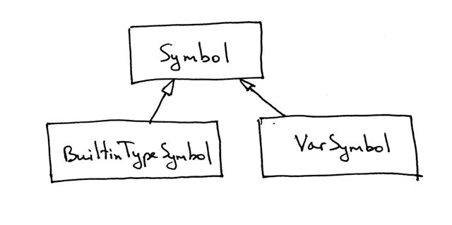
    Here is the hierarchy of symbols we’ve defined in visual form:

    So far so good, but we haven’t answered the question yet as to why we even need to track those symbols in the first place.

    Here are some of the reasons:

    • To make sure that when we assign a value to a variable the types are correct (type checking)
    • To make sure that a variable is declared before it is used

    Take a look at the following incorrect Pascal program, for example:

    There are two problems with the program above (you can compile it with fpc to see it for yourself):

    1. In the expression “x := 2 + y;” we assigned a decimal value to the variable “x” that was declared as integer. That wouldn’t compile because the types are incompatible.
    2. In the assignment statement “x := a;” we referenced the variable “a” that wasn’t declared - wrong!

    To be able to identify cases like that even before interpreting/evaluating the source code of the program at run-time, we need to track program symbols. And where do we store the symbols that we track? I think you’ve guessed it right - in the symbol table!

    What is a symbol table? A symbol table is an abstract data type (ADT) for tracking various symbols in source code. Today we’re going to implement our symbol table as a separate class with some helper methods:

    classSymbolTable(object):def__init__(self):self._symbols=OrderedDict()def__str__(self):s='Symbols: {symbols}'.format(symbols=[valueforvalueinself._symbols.values()])returns__repr__=__str__defdefine(self,symbol):print('Define: %s'%symbol)self._symbols[symbol.name]=symboldeflookup(self,name):print('Lookup: %s'%name)symbol=self._symbols.get(name)# 'symbol' is either an instance of the Symbol class or 'None'returnsymbol

    There are two main operations that we will be performing with the symbol table: storing symbols and looking them up by name: hence, we need two helper methods - define and lookup.

    The method define takes a symbol as a parameter and stores it internally in its _symbols ordered dictionary using the symbol’s name as a key and the symbol instance as a value. The method lookup takes a symbol name as a parameter and returns a symbol if it finds it or “None” if it doesn’t.

    Let’s manually populate our symbol table for the same Pascal program we’ve used just recently where we were manually creating variable and built-in type symbols:

    PROGRAMPart11;VARx:INTEGER;y:REAL;BEGINEND.

    Launch a Python shell again and follow along:

    $ python
    >>> from spi import SymbolTable, BuiltinTypeSymbol, VarSymbol
    >>> symtab= SymbolTable()>>> int_type= BuiltinTypeSymbol('INTEGER')>>> symtab.define(int_type)
    Define: INTEGER
    >>> symtab
    Symbols: [INTEGER]>>>
    >>> var_x_symbol= VarSymbol('x', int_type)>>> symtab.define(var_x_symbol)
    Define: <x:INTEGER>
    >>> symtab
    Symbols: [INTEGER, <x:INTEGER>]>>>
    >>> real_type= BuiltinTypeSymbol('REAL')>>> symtab.define(real_type)
    Define: REAL
    >>> symtab
    Symbols: [INTEGER, <x:INTEGER>, REAL]>>>
    >>> var_y_symbol= VarSymbol('y', real_type)>>> symtab.define(var_y_symbol)
    Define: <y:REAL>
    >>> symtab
    Symbols: [INTEGER, <x:INTEGER>, REAL, <y:REAL>]

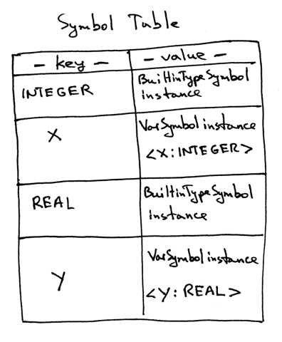
    If you looked at the contents of the _symbols dictionary it would look something like this:

    How do we automate the process of building the symbol table? We’ll just write another node visitor that walks the AST built by our parser! This is another example of how useful it is to have an intermediary form like AST. Instead of extending our parser to deal with the symbol table, we separate concerns and write a new node visitor class. Nice and clean. :)

    Before doing that, though, let’s extend our SymbolTable class to initialize the built-in types when the symbol table instance is created. Here is the full source code for today’s SymbolTable class:

    classSymbolTable(object):def__init__(self):self._symbols=OrderedDict()self._init_builtins()def_init_builtins(self):self.define(BuiltinTypeSymbol('INTEGER'))self.define(BuiltinTypeSymbol('REAL'))def__str__(self):s='Symbols: {symbols}'.format(symbols=[valueforvalueinself._symbols.values()])returns__repr__=__str__defdefine(self,symbol):print('Define: %s'%symbol)self._symbols[symbol.name]=symboldeflookup(self,name):print('Lookup: %s'%name)symbol=self._symbols.get(name)# 'symbol' is either an instance of the Symbol class or 'None'returnsymbol

    Now onto the SymbolTableBuilderAST node visitor:

    classSymbolTableBuilder(NodeVisitor):def__init__(self):self.symtab=SymbolTable()defvisit_Block(self,node):fordeclarationinnode.declarations:self.visit(declaration)self.visit(node.compound_statement)defvisit_Program(self,node):self.visit(node.block)defvisit_BinOp(self,node):self.visit(node.left)self.visit(node.right)defvisit_Num(self,node):passdefvisit_UnaryOp(self,node):self.visit(node.expr)defvisit_Compound(self,node):forchildinnode.children:self.visit(child)defvisit_NoOp(self,node):passdefvisit_VarDecl(self,node):type_name=node.type_node.valuetype_symbol=self.symtab.lookup(type_name)var_name=node.var_node.valuevar_symbol=VarSymbol(var_name,type_symbol)self.symtab.define(var_symbol)

    You’ve seen most of those methods before in the Interpreter class, but the visit_VarDecl method deserves some special attention. Here it is again:

    defvisit_VarDecl(self,node):type_name=node.type_node.valuetype_symbol=self.symtab.lookup(type_name)var_name=node.var_node.valuevar_symbol=VarSymbol(var_name,type_symbol)self.symtab.define(var_symbol)

    This method is responsible for visiting (walking) a VarDeclAST node and storing the corresponding symbol in the symbol table. First, the method looks up the built-in type symbol by name in the symbol table, then it creates an instance of the VarSymbol class and stores (defines) it in the symbol table.

    Let’s take our SymbolTableBuilderAST walker for a test drive and see it in action:

    $ python
    >>> from spi import Lexer, Parser, SymbolTableBuilder
    >>> text="""... PROGRAM Part11;... VAR...    x : INTEGER;...    y : REAL;...... BEGIN...... END.... """>>> lexer= Lexer(text)>>> parser= Parser(lexer)>>> tree= parser.parse()>>> symtab_builder= SymbolTableBuilder()
    Define: INTEGER
    Define: REAL
    >>> symtab_builder.visit(tree)
    Lookup: INTEGER
    Define: <x:INTEGER>
    Lookup: REAL
    Define: <y:REAL>
    >>> # Let’s examine the contents of our symbol table…
    >>> symtab_builder.symtab
    Symbols: [INTEGER, REAL, <x:INTEGER>, <y:REAL>]

    In the interactive session above, you can see the sequence of “Define: …” and “Lookup: …” messages that indicate the order in which symbols are defined and looked up in the symbol table. The last command in the session prints the contents of the symbol table and you can see that it’s exactly the same as the contents of the symbol table that we’ve built manually before. The magic of AST node visitors is that they pretty much do all the work for you. :)

    We can already put our symbol table and symbol table builder to good use: we can use them to verify that variables are declared before they are used in assignments and expressions. All we need to do is just extend the visitor with two more methods: visit_Assign and visit_Var:

    defvisit_Assign(self,node):var_name=node.left.valuevar_symbol=self.symtab.lookup(var_name)ifvar_symbolisNone:raiseNameError(repr(var_name))self.visit(node.right)defvisit_Var(self,node):var_name=node.valuevar_symbol=self.symtab.lookup(var_name)ifvar_symbolisNone:raiseNameError(repr(var_name))

    These methods will raise a NameError exception if they cannot find the symbol in the symbol table.

    Take a look at the following program, where we reference the variable “b” that hasn’t been declared yet:

    PROGRAMNameError1;VARa:INTEGER;BEGINa:=2+b;END.

    Let’s see what happens if we construct an AST for the program and pass it to our symbol table builder to visit:

    $ python
    >>> from spi import Lexer, Parser, SymbolTableBuilder
    >>> text="""... PROGRAM NameError1;... VAR...    a : INTEGER;...... BEGIN...    a := 2 + b;... END.... """>>> lexer= Lexer(text)>>> parser= Parser(lexer)>>> tree= parser.parse()>>> symtab_builder= SymbolTableBuilder()
    Define: INTEGER
    Define: REAL
    >>> symtab_builder.visit(tree)
    Lookup: INTEGER
    Define: <a:INTEGER>
    Lookup: a
    Lookup: b
    Traceback (most recent call last):
      ...
      File "spi.py", line 674, in visit_Var
        raise NameError(repr(var_name))
    NameError: 'b'

    Exactly what we were expecting!

    Here is another error case where we try to assign a value to a variable that hasn’t been defined yet, in this case the variable ‘a’:

    PROGRAMNameError2;VARb:INTEGER;BEGINb:=1;a:=b+2;END.

    Meanwhile, in the Python shell:

    >>> from spi import Lexer, Parser, SymbolTableBuilder
    >>> text="""... PROGRAM NameError2;... VAR...    b : INTEGER;...... BEGIN...    b := 1;...    a := b + 2;... END.... """>>> lexer= Lexer(text)>>> parser= Parser(lexer)>>> tree= parser.parse()>>> symtab_builder= SymbolTableBuilder()
    Define: INTEGER
    Define: REAL
    >>> symtab_builder.visit(tree)
    Lookup: INTEGER
    Define: <b:INTEGER>
    Lookup: b
    Lookup: a
    Traceback (most recent call last):
      ...
      File "spi.py", line 665, in visit_Assign
        raise NameError(repr(var_name))
    NameError: 'a'

    Great, our new visitor caught this problem too!

    I would like to emphasize the point that all those checks that our SymbolTableBuilderAST visitor makes are made before the run-time, so before our interpreter actually evaluates the source program. To drive the point home if we were to interpret the following program:

    PROGRAMPart11;VARx:INTEGER;BEGINx:=2;END.

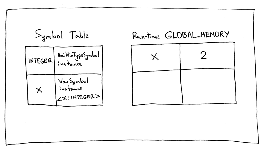
    The contents of the symbol table and the run-time GLOBAL_MEMORY right before the program exited would look something like this:

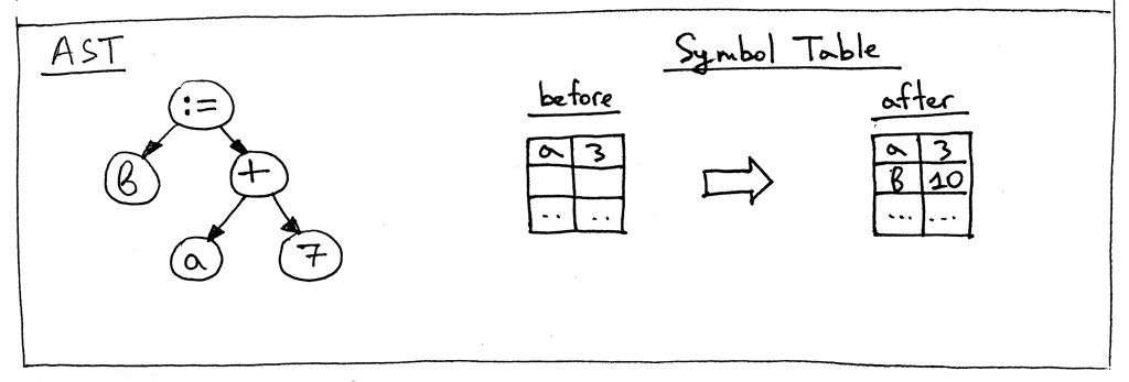
    Do you see the difference? Can you see that the symbol table doesn’t hold the value 2 for variable “x”? That’s solely the interpreter’s job now.

    Remember the picture from Part 9 where the Symbol Table was used as global memory?

    No more! We effectively got rid of the hack where symbol table did double duty as global memory.

    Let’s put it all together and test our new interpreter with the following program:

    PROGRAMPart11;VARnumber:INTEGER;a,b:INTEGER;y:REAL;BEGIN{Part11}number:=2;a:=number;b:=10*a+10*numberDIV4;y:=20/7+3.14END.{Part11}

    Save the program as part11.pas and fire up the interpreter:

    $ python spi.py part11.pas
    Define: INTEGER
    Define: REAL
    Lookup: INTEGER
    Define: <number:INTEGER>
    Lookup: INTEGER
    Define: <a:INTEGER>
    Lookup: INTEGER
    Define: <b:INTEGER>
    Lookup: REAL
    Define: <y:REAL>
    Lookup: number
    Lookup: a
    Lookup: number
    Lookup: b
    Lookup: a
    Lookup: number
    Lookup: y
    
    Symbol Table contents:
    Symbols: [INTEGER, REAL, <number:INTEGER>, <a:INTEGER>, <b:INTEGER>, <y:REAL>]
    
    Run-time GLOBAL_MEMORY contents:
    a= 2
    b= 25
    number= 2
    y= 5.99714285714
    

    I’d like to draw your attention again to the fact that the Interpreter class has nothing to do with building the symbol table and it relies on the SymbolTableBuilder to make sure that the variables in the source code are properly declared before they are used by the Interpreter.

    Check your understanding

    • What is a symbol?
    • Why do we need to track symbols?
    • What is a symbol table?
    • What is the difference between defining a symbol and resolving/looking up the symbol?
    • Given the following small Pascal program, what would be the contents of the symbol table, the global memory (the GLOBAL_MEMORY dictionary that is part of the Interpreter)?
      PROGRAMPart11;VARx,y:INTEGER;BEGINx:=2;y:=3+x;END.

    That’s all for today. In the next article, I’ll talk about scopes and we’ll get our hands dirty with parsing nested procedures. Stay tuned and see you soon! And remember that no matter what, “Keep going!”

    P.S. My explanation of the topic of symbols and symbol table management is heavily influenced by the book Language Implementation Patterns by Terence Parr. It’s a terrific book. I think it has the clearest explanation of the topic I’ve ever seen and it also covers class scopes, a subject that I’m not going to cover in the series because we will not be discussing object-oriented Pascal.

    P.P.S.: If you can’t wait and want to start digging into compilers, I highly recommend the freely available classic by Jack Crenshaw “Let’s Build a Compiler.”


    By the way, I’m writing a book “Let’s Build A Web Server: First Steps” that explains how to write a basic web server from scratch. You can get a feel for the book here, here, and here. Subscribe to the mailing list to get the latest updates about the book and the release date.

    OPTIN_FORM_PLACEHOLDER


    All articles in this series:

    tryexceptpass: On Democratizing the Next Generation of User Interfaces

    Codementor: Image Manipulation in Python

    $
    0
    0

    Color Space Background

    CMYK Color Representation:

    When we see a printed advertisement or poster, the colors are printed with color spaces based on the CMYK color model, using the subtractive primary colors of pigment Cyan, Magenta, Yellow, and blacK. This is also known as the four-colors print process.

    python image processing

    The “primary” and “secondary” colors in a four-color print process are exhibited below.

    python image processing

    RGB Color Representation:

    While printed colors are represented with the use of the four-color process, monitors represent color using the RGB color model which is an additive color model in which Red, Green and Blue light are added together in various ways to reproduce a broad array of colors.

    python image processing

    The Difference Between Print and Monitor Color

    Offset lithography is one of the most common ways of creating printed materials. A few of its applications include newspapers, magazines, brochures, stationery, and books. This model requires the image to be converted or made in the CMYK color model. All printed material relies on creating pigments of colors that when combined, forms the color as shown below.

    python image processing

    The ink’s semi-opacity property is in conjunction with the halftone technology and this is responsible for allowing pigments to mix and create new colors with just four primary ones.

    On the other hand, media that transmit light (such as the monitor on your PC, tablet, or phone) use additive color mixing, which means that every pixel is made from three colors (RGB color model) by displaying different intensity the colors get produced.

    Why Should I Care?

    The first thing you might be wondering is why am I telling you how traditional press works, the existence of CMYK and RGB color models, or the pigment process (ink opacity plus halftoning) to print a brochure.

    The rest of the tutorial will show you how to transform an image with different filters and techniques to deliver different outputs. These methods are still in use and part of a process known as Computer-To-Plate (CTP), used to create a direct output from an image file to a photographic film or plate (depending on the process), which are employed in industrial machines like the ones from Heidelberg.

    This tutorial will give you insight into the filters and techniques used to transform images, some international image standards, and hopefully, some interest in the history of printing.

    Quick Notes

    1. Pillow is a fork of PIL (Python Imaging Library)
    2. Pillow and PIL cannot co-exist in the same environment. Before installing Pillow, uninstall PIL.
    3. libjpeg-dev is required to be able to process jpeg’s with Pillow.
    4. Pillow >= 2.0.0 supports Python versions 2.6, 2.7, 3.2, 3.3, and 3.4
    5. Pillow >= 1.0 no longer supports import Image. Use from PIL import Image instead.

    Installing Required Library

    Before we start, we will need Python 3 and Pillow. If you are using Linux, Pillow will probably be there already, since major distributions including Fedora, Debian/Ubuntu, and ArchLinux include Pillow in packages that previously contained PIL.

    The easiest way to install it is to use pip:

    pip install Pillow
    

    The installation process should look similar to the following.

    python image processing

    If any trouble happens, I recommend reading the documentation from the Pillow Manual.

    Basic Methods

    Before manipulating an image, we need to be able to open the file, save the changes, create an empty picture, and to obtain individual pixels color. For the convenience of this tutorial, I have already made the methods to do so, which will be used in all subsequent sections.

    These methods rely on the imported image library from the Pillow package.

    # Imported PIL Library
    from PIL import Image


    # Open an Image
    def open_image(path):
        newImage = Image.open(path)
        return newImage


    # Save Image
    def save_image(image, path):
        image.save(path, 'png')


    # Create a new image with the given size
    def create_image(i, j):
        image = Image.new("RGB", (i, j), "white")
        return image


    # Get the pixel from the given image
    def get_pixel(image, i, j):
        # Inside image bounds?
        width, height = image.size
        if i > width or j > height:
            return None
    
        # Get Pixel
        pixel = image.getpixel((i, j))
        return pixel

    Grayscale Filter

    The traditional grayscale algorithm transforms an image to grayscale by obtaining the average channels color and making each channel equals to the average.

    python image processing

    A better choice for grayscale is the ITU-R Recommendation BT.601-7, which specifies methods for digitally coding video signals by normalizing the values. For the grayscale transmissions, it defines the following formula.

    BT.601-7

    # Create a Grayscale version of the image
    def convert_grayscale(image):
        # Get size
        width, height = image.size
    
        # Create new Image and a Pixel Map
        new = create_image(width, height)
        pixels = new.load()
    
        # Transform to grayscale
        for i in range(width):
            for j in range(height):
                # Get Pixel
                pixel = get_pixel(image, i, j)
    
                # Get R, G, B values (This are int from 0 to 255)
                red =   pixel[0]
                green = pixel[1]
                blue =  pixel[2]
    
                # Transform to grayscale
                gray = (red * 0.299) + (green * 0.587) + (blue * 0.114)
    
                # Set Pixel in new image
                pixels[i, j] = (int(gray), int(gray), int(gray))
    
        # Return new image
        return new

    By applying the filter with the above code, and using the BT.601-7 recommendation, we get the following result.

    python image processing

    Half-tone Filter

    The halftoning filter is the traditional method of printing images. It is a reprographic technique that simulates continuous tone imagery through the use of dots.

    To generate the effect of shades of gray using only dots of black, we will define a size, in this case, a two by two matrix, and depending on the saturation we will draw black dots in this matrix.

    # Create a Half-tone version of the image
    def convert_halftoning(image):
        # Get size
        width, height = image.size
    
        # Create new Image and a Pixel Map
        new = create_image(width, height)
        pixels = new.load()
    
        # Transform to half tones
        for i in range(0, width, 2):
            for j in range(0, height, 2):
                # Get Pixels
                p1 = get_pixel(image, i, j)
                p2 = get_pixel(image, i, j + 1)
                p3 = get_pixel(image, i + 1, j)
                p4 = get_pixel(image, i + 1, j + 1)
    
                # Transform to grayscale
                gray1 = (p1[0] * 0.299) + (p1[1] * 0.587) + (p1[2] * 0.114)
                gray2 = (p2[0] * 0.299) + (p2[1] * 0.587) + (p2[2] * 0.114)
                gray3 = (p3[0] * 0.299) + (p3[1] * 0.587) + (p3[2] * 0.114)
                gray4 = (p4[0] * 0.299) + (p4[1] * 0.587) + (p4[2] * 0.114)
    
                # Saturation Percentage
                sat = (gray1 + gray2 + gray3 + gray4) / 4
    
                # Draw white/black depending on saturation
                if sat > 223:
                    pixels[i, j]         = (255, 255, 255) # White
                    pixels[i, j + 1]     = (255, 255, 255) # White
                    pixels[i + 1, j]     = (255, 255, 255) # White
                    pixels[i + 1, j + 1] = (255, 255, 255) # White
                elif sat > 159:
                    pixels[i, j]         = (255, 255, 255) # White
                    pixels[i, j + 1]     = (0, 0, 0)       # Black
                    pixels[i + 1, j]     = (255, 255, 255) # White
                    pixels[i + 1, j + 1] = (255, 255, 255) # White
                elif sat > 95:
                    pixels[i, j]         = (255, 255, 255) # White
                    pixels[i, j + 1]     = (0, 0, 0)       # Black
                    pixels[i + 1, j]     = (0, 0, 0)       # Black
                    pixels[i + 1, j + 1] = (255, 255, 255) # White
                elif sat > 32:
                    pixels[i, j]         = (0, 0, 0)       # Black
                    pixels[i, j + 1]     = (255, 255, 255) # White
                    pixels[i + 1, j]     = (0, 0, 0)       # Black
                    pixels[i + 1, j + 1] = (0, 0, 0)       # Black
                else:
                    pixels[i, j]         = (0, 0, 0)       # Black
                    pixels[i, j + 1]     = (0, 0, 0)       # Black
                    pixels[i + 1, j]     = (0, 0, 0)       # Black
                    pixels[i + 1, j + 1] = (0, 0, 0)       # Black
    
        # Return new image
        return new

    By applying the filter using the code above, we are separating in five ranges and coloring the pixels on the array white or black depending on the saturation, which will produce the following result.

    python image processing

    Dithering Filter

    Dithering is an intentionally applied form of noise; it is used for processing an image to generate the illusion of colors by using the halftone filter on each color channel.

    This method is used in traditional print as explained earlier.
    In our approach, we will set the saturation for each channel,
    in a direct fashion by replicating the halftone algorithm in each channel.
    For a more advanced dither filter, you can read about the Floyd–Steinberg dithering.

    # Return color value depending on quadrant and saturation
    def get_saturation(value, quadrant):
        if value > 223:
            return 255
        elif value > 159:
            if quadrant != 1:
                return 255
    
            return 0
        elif value > 95:
            if quadrant == 0 or quadrant == 3:
                return 255
    
            return 0
        elif value > 32:
            if quadrant == 1:
                return 255
    
            return 0
        else:
            return 0


    # Create a dithered version of the image
    def convert_dithering(image):
        # Get size
        width, height = image.size
    
        # Create new Image and a Pixel Map
        new = create_image(width, height)
        pixels = new.load()
    
        # Transform to half tones
        for i in range(0, width, 2):
            for j in range(0, height, 2):
                # Get Pixels
                p1 = get_pixel(image, i, j)
                p2 = get_pixel(image, i, j + 1)
                p3 = get_pixel(image, i + 1, j)
                p4 = get_pixel(image, i + 1, j + 1)
    
                # Color Saturation by RGB channel
                red   = (p1[0] + p2[0] + p3[0] + p4[0]) / 4
                green = (p1[1] + p2[1] + p3[1] + p4[1]) / 4
                blue  = (p1[2] + p2[2] + p3[2] + p4[2]) / 4
    
                # Results by channel
                r = [0, 0, 0, 0]
                g = [0, 0, 0, 0]
                b = [0, 0, 0, 0]
    
                # Get Quadrant Color
                for x in range(0, 4):
                    r[x] = get_saturation(red, x)
                    g[x] = get_saturation(green, x)
                    b[x] = get_saturation(blue, x)
    
                # Set Dithered Colors
                pixels[i, j]         = (r[0], g[0], b[0])
                pixels[i, j + 1]     = (r[1], g[1], b[1])
                pixels[i + 1, j]     = (r[2], g[2], b[2])
                pixels[i + 1, j + 1] = (r[3], g[3], b[3])
    
        # Return new image
        return new

    By processing each channel, we set the colors to the primary and secondary ones. This is a total of eight colors, but as you notice in the processed image, they give the illusion of a wider array of colors.

    python image processing

    Complete Source

    The complete code to process images takes a PNG file in RGB color mode (with no transparency), saving the output as different images.

    Due to limitations with JPEG support on various operating systems, I choose the PNG format.

    '''
        This Example opens an Image and transform the image into grayscale, halftone, dithering, and primary colors.
        You need PILLOW (Python Imaging Library fork) and Python 3.5
        -Isai B. Cicourel
    '''
    
    
    # Imported PIL Library
    from PIL import Image


    # Open an Image
    def open_image(path):
        newImage = Image.open(path)
        return newImage


    # Save Image
    def save_image(image, path):
        image.save(path, 'png')


    # Create a new image with the given size
    def create_image(i, j):
        image = Image.new("RGB", (i, j), "white")
        return image


    # Get the pixel from the given image
    def get_pixel(image, i, j):
        # Inside image bounds?
        width, height = image.size
        if i > width or j > height:
            return None
    
        # Get Pixel
        pixel = image.getpixel((i, j))
        return pixel


    # Create a Grayscale version of the image
    def convert_grayscale(image):
        # Get size
        width, height = image.size
    
        # Create new Image and a Pixel Map
        new = create_image(width, height)
        pixels = new.load()
    
        # Transform to grayscale
        for i in range(width):
            for j in range(height):
                # Get Pixel
                pixel = get_pixel(image, i, j)
    
                # Get R, G, B values (This are int from 0 to 255)
                red =   pixel[0]
                green = pixel[1]
                blue =  pixel[2]
    
                # Transform to grayscale
                gray = (red * 0.299) + (green * 0.587) + (blue * 0.114)
    
                # Set Pixel in new image
                pixels[i, j] = (int(gray), int(gray), int(gray))
    
        # Return new image
        return new


    # Create a Half-tone version of the image
    def convert_halftoning(image):
        # Get size
        width, height = image.size
    
        # Create new Image and a Pixel Map
        new = create_image(width, height)
        pixels = new.load()
    
        # Transform to half tones
        for i in range(0, width, 2):
            for j in range(0, height, 2):
                # Get Pixels
                p1 = get_pixel(image, i, j)
                p2 = get_pixel(image, i, j + 1)
                p3 = get_pixel(image, i + 1, j)
                p4 = get_pixel(image, i + 1, j + 1)
    
                # Transform to grayscale
                gray1 = (p1[0] * 0.299) + (p1[1] * 0.587) + (p1[2] * 0.114)
                gray2 = (p2[0] * 0.299) + (p2[1] * 0.587) + (p2[2] * 0.114)
                gray3 = (p3[0] * 0.299) + (p3[1] * 0.587) + (p3[2] * 0.114)
                gray4 = (p4[0] * 0.299) + (p4[1] * 0.587) + (p4[2] * 0.114)
    
                # Saturation Percentage
                sat = (gray1 + gray2 + gray3 + gray4) / 4
    
                # Draw white/black depending on saturation
                if sat > 223:
                    pixels[i, j]         = (255, 255, 255) # White
                    pixels[i, j + 1]     = (255, 255, 255) # White
                    pixels[i + 1, j]     = (255, 255, 255) # White
                    pixels[i + 1, j + 1] = (255, 255, 255) # White
                elif sat > 159:
                    pixels[i, j]         = (255, 255, 255) # White
                    pixels[i, j + 1]     = (0, 0, 0)       # Black
                    pixels[i + 1, j]     = (255, 255, 255) # White
                    pixels[i + 1, j + 1] = (255, 255, 255) # White
                elif sat > 95:
                    pixels[i, j]         = (255, 255, 255) # White
                    pixels[i, j + 1]     = (0, 0, 0)       # Black
                    pixels[i + 1, j]     = (0, 0, 0)       # Black
                    pixels[i + 1, j + 1] = (255, 255, 255) # White
                elif sat > 32:
                    pixels[i, j]         = (0, 0, 0)       # Black
                    pixels[i, j + 1]     = (255, 255, 255) # White
                    pixels[i + 1, j]     = (0, 0, 0)       # Black
                    pixels[i + 1, j + 1] = (0, 0, 0)       # Black
                else:
                    pixels[i, j]         = (0, 0, 0)       # Black
                    pixels[i, j + 1]     = (0, 0, 0)       # Black
                    pixels[i + 1, j]     = (0, 0, 0)       # Black
                    pixels[i + 1, j + 1] = (0, 0, 0)       # Black
    
        # Return new image
        return new


    # Return color value depending on quadrant and saturation
    def get_saturation(value, quadrant):
        if value > 223:
            return 255
        elif value > 159:
            if quadrant != 1:
                return 255
    
            return 0
        elif value > 95:
            if quadrant == 0 or quadrant == 3:
                return 255
    
            return 0
        elif value > 32:
            if quadrant == 1:
                return 255
    
            return 0
        else:
            return 0


    # Create a dithered version of the image
    def convert_dithering(image):
        # Get size
        width, height = image.size
    
        # Create new Image and a Pixel Map
        new = create_image(width, height)
        pixels = new.load()
    
        # Transform to half tones
        for i in range(0, width, 2):
            for j in range(0, height, 2):
                # Get Pixels
                p1 = get_pixel(image, i, j)
                p2 = get_pixel(image, i, j + 1)
                p3 = get_pixel(image, i + 1, j)
                p4 = get_pixel(image, i + 1, j + 1)
    
                # Color Saturation by RGB channel
                red   = (p1[0] + p2[0] + p3[0] + p4[0]) / 4
                green = (p1[1] + p2[1] + p3[1] + p4[1]) / 4
                blue  = (p1[2] + p2[2] + p3[2] + p4[2]) / 4
    
                # Results by channel
                r = [0, 0, 0, 0]
                g = [0, 0, 0, 0]
                b = [0, 0, 0, 0]
    
                # Get Quadrant Color
                for x in range(0, 4):
                    r[x] = get_saturation(red, x)
                    g[x] = get_saturation(green, x)
                    b[x] = get_saturation(blue, x)
    
                # Set Dithered Colors
                pixels[i, j]         = (r[0], g[0], b[0])
                pixels[i, j + 1]     = (r[1], g[1], b[1])
                pixels[i + 1, j]     = (r[2], g[2], b[2])
                pixels[i + 1, j + 1] = (r[3], g[3], b[3])
    
        # Return new image
        return new


    # Create a Primary Colors version of the image
    def convert_primary(image):
        # Get size
        width, height = image.size
    
        # Create new Image and a Pixel Map
        new = create_image(width, height)
        pixels = new.load()
    
        # Transform to primary
        for i in range(width):
            for j in range(height):
                # Get Pixel
                pixel = get_pixel(image, i, j)
    
                # Get R, G, B values (This are int from 0 to 255)
                red =   pixel[0]
                green = pixel[1]
                blue =  pixel[2]
    
                # Transform to primary
                if red > 127:
                    red = 255
                else:
                    red = 0
                if green > 127:
                    green = 255
                else:
                    green = 0
                if blue > 127:
                    blue = 255
                else:
                    blue = 0
    
                # Set Pixel in new image
                pixels[i, j] = (int(red), int(green), int(blue))
    
        # Return new image
        return new


    # Main
    if __name__ == "__main__":
        # Load Image (JPEG/JPG needs libjpeg to load)
        original = open_image('Hero_Prinny.png')
    
        # Example Pixel Color
        print('Color: ' + str(get_pixel(original, 0, 0)))
    
        # Convert to Grayscale and save
        new = convert_grayscale(original)
        save_image(new, 'Prinny_gray.png')
    
        # Convert to Halftoning and save
        new = convert_halftoning(original)
        save_image(new, 'Prinny_half.png')
    
        # Convert to Dithering and save
        new = convert_dithering(original)
        save_image(new, 'Prinny_dither.png')
    
        # Convert to Primary and save
        new = convert_primary(original)
        save_image(new, 'Prinny_primary.png')

    The source code takes an image, then applies each filter and saves the output as a new image, producing the following results.

    Don’t forget to specify the path to the image in original = open_image('Hero_Prinny.png') and on the outputs. Unless you have that image, which would mean you are a Disgaea fan.

    python image processing

    Wrapping Up

    Image filters are not only something we use to make our pictures on social networking sites look cool, they are useful and powerful techniques for processing videos and images not only for printing in an offset; but also to compress and improve playback and speed of on-demand services.

    Have You Tried The Following?

    Now that you know some image filters, how about applying several of them on the same picture?

    On a large image, what happens with a filter when you “fit to screen”?

    Did you notice the extra filter in the complete source code?

    Have you checked the size of the different output images?

    Play around and check what happens. Create your filter or implement a new one, the idea is to learn new things. If you like this tutorial, share it with your friends. ;-)


    ##Other tutorials you might be interested in:

    Martijn Faassen: Is Morepath Fast Yet?

    $
    0
    0

    Morepath is a Python web framework. But is it fast enough for your purposes?

    Does performance matter?

    Performance is one of the least important criteria you should use when you pick a Python web framework. You're using Python for web development after all; you are already compromising performance for ease of use.

    But performance makes things seem easy. It boils down the whole choice between web frameworks to a single seemingly easy to understand variable: how fast is this thing? All web frameworks are the same anyway, right? (Wrong). We don't want the speed of our application be dragged down by the web framework. So we should just pick the one that is fastest. Makes total sense.

    It makes total sense until you take a few minutes to think about it. Performance, sure, but performance doing what? Performance is notoriously difficult to measure. Sending a single "hello world" response? Parsing complex URLs with multiple variables in them? HTML template rendering? JSON serialization? Link generation? What aspect of performance matters to you depends on the application you're building. Why do we worry so much about performance and not about features, anyway?

    Choosing a web framework based on performance makes no sense for most people. For most applications, application code dominates the CPU time spent. Pulling stuff out of a database can take vastly more time than rendering a web response.

    What matters

    So it makes sense to look at other factors when picking a web framework. Is there documentation? Can it do what I need it to do? Will it grow with me over time? Is it flexible? Is it being maintained? What's the community like? Does it have a cool logo?

    Okay, I'm starting to sound like someone who doesn't want to admit the web framework I work on, Morepath, is atrociously slow. I'm giving you all kinds of reasons why you should use it despite its performance, which you would guess is pretty atrocious. It's true that the primary selling point of Morepath isn't performance -- it's flexibility. It's a micro-framework that is easy to learn but that doesn't let you down when your requirements become more complex.

    Morepath performance

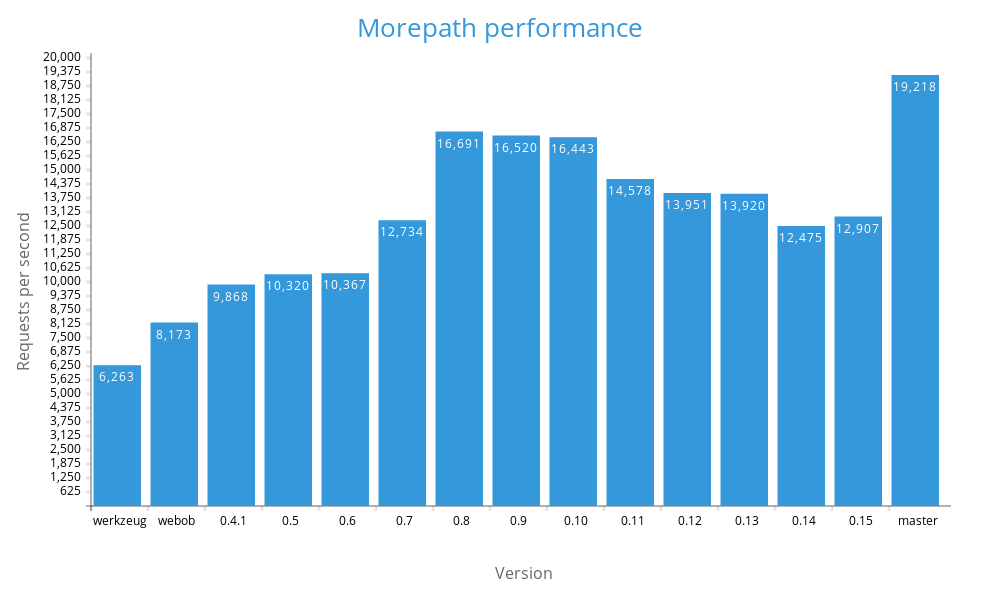
    I maintain a very simple benchmark tool that measures just one aspect of performance: how fast a web framework at the Python WSGI level can generate simple "hello world" responses.

    https://github.com/faassen/welcome-bench

    I run it against Morepath once every while to see how we're doing with performance. I actually care more about what the framework is doing when Morepath generates the response than I care about the actual requests per second it can generate. I want Morepath's underlying complexity to be relatively simple. But since performance is so easy to think about I take advantage of that as a shortcut. I treat performance as an approximation of implementation complexity. Plus it's cool when your framework is fast, I admit it.

    The current Morepath development version takes about 5200 ms per request, which translates to about 19200 requests per second. Let's see how that compares to some of the friendly competition:

                    ms     rps  tcalls  funcs
    django       10992    9098     190     85
    flask        15854    6308     270    125
    morepath      5204   19218     109     80
    

    So at this silly benchmark, Morepath is more than twice as fast as Django and more than three times faster than Flask!

    Let me highlight that for marketing purposes and trick those who aren't reading carefully:

    Morepath is more than 2 times faster than Django and more than 3 times faster than Flask

    Yay! End of story. Well, I gave a bit of a selective view just now. Here are some other web frameworks:

                    ms     rps  tcalls  funcs
    bottle        2172   46030      53     31
    falcon        1539   64961      26     24
    morepath      5204   19218     109     80
    pyramid       3920   25509      72     57
    wheezy.web    1201   83247      25     23
    

    I'm not going to highlight that Bottle is more than two times faster at this silly benchmark nor that Falcon is more than three times faster. Let's not even think about wheezy.web.

    I think this performance comparison actually highlights my point that in practice web framework performance is usually irrelevant. People aren't flocking to wheezy.web just because it's so fast. People aren't ignoring Flask because it's comparatively slow. I suspect many are surprised are surprised Flask is one of the slowest frameworks in this benchmark, as it's a lightweight framework.

    Flask's relatively slow performance hasn't hurt its popularity. This demonstrates my point that web framework performance isn't that important overall. I don't fully understand why Flask is relatively slow, but I know part of the reason is werkzeug, its request/response implementation. Morepath is actually doing a lot more sophisticated stuff underneath than Flask and it's still faster. That Pyramid is faster than Morepath is impressive, as what it needs to do during runtime is similar to Morepath.

    Let's look at the tcalls column: how many function calls get executed during a request. There is a strong correlation between how many Python function calls there are during a request and requests per second. This is why performance is a decent approximation of implementation complexity. It's also a clear sign we're using an interpreted language.

    How Morepath performance has changed

    So how has Morepath's performance evolved over time? Here's a nice graph:

    Morepath performance over time

    So what does this chart tell us? Before it's 0.1 release when it still used werkzeug, Morepath was actually about as slow as Flask. After we switched to webob, Morepath became faster than Flask, but was still slower than Django.

    By release 0.4.1 a bunch of minor improvements had pushed performance slightly beyond Django's -- but I don't have a clear idea of the details. I also don't understand exactly why there's a performance bump for 0.7, though I suspect it has to do with a refactor of application mounting behavior I did around that time -- while that code isn't exercised in this benchmark, it's possible it simplified a critical path.

    I do know what caused the huge bump in performance in 0.8. This marked the switch to Reg 0.9, which is a dispatch library that is used heavily by Morepath. Reg 0.9 got faster, as this is when Reg switched to a more flexible and efficient predicate dispatch approach.

    Performance was stable again until version 0.11, when it went down again. In 0.11 we introduced a measure to make the request object sanitize potentially dangerous input, and this cost us some performance. I'm not sure what caused the slight performance drop in 0.14.

    And then there's a vast performance increase in current master. What explains this? Two things:

    • We've made some huge improvements to Reg again. Morepath benefits because it uses Reg heavily.
    • I cheated. That is, I found work that could be skipped in the case no URL parameters are in play, as in this benchmark.

    Skipping unnecessary work was a legitimate improvement of Morepath. The code now avoids accessing the relatively expensive GET attribute on the webob request, and also avoids a for loop through an empty list and a few if statements. In Python, performance is sensitive to even a few extra lines of code on the critical path.

    But when you do have URL parameters, Morepath's feature that lets you convert and validate them automatically is pretty nice -- in almost all circumstances you should be glad to pay the slight performance penalty for the convenience. Features are usually worth their performance cost.

    So is Morepath fast yet?

    Is Morepath fast yet? Probably. Does it matter? It depends. What benchmark? But for those just skimming this article, I'll do another sneaky highlight:

    Morepath is fast. Morepath outperforms the most popular Python web frameworks while offering a lot more flexibility.

    Kushal Das: Dgplug contributor grant recipient Trishna Guha

    $
    0
    0

    I am happy to announce that Trishna Guha is the recipient of a dgplug contributor grant for 2016. She is an upstream contributor in Fedora Cloud SIG, and hacks on Bodhi in her free time. Trishna started her open source journey just a year back during the dgplug summer training 2015, you can read more about her work in a previous blog post. She has also become an active member of the local Pune PyLadies chapter.

    The active members of dgplug.org every year contribute funding, which we then use to help out community members as required. For example, we previously used this fund to pay accommodation costs for our women contributors during PyCon. This year we are happy to be able to assist Trishna Guha to attend PyCon India 2016. Her presence and expertise with upstream development will help diversity efforts at various levels. As she is still a college student, we found many students are interested to talk to and learn from her. So, if you are coming down to PyCon India this weekend, remember to visit the Red Hat booth, and have a chat with Trishna.

    Matthew Rocklin: Dask Cluster Deployments

    $
    0
    0

    This work is supported by Continuum Analytics and the XDATA Program as part of the Blaze Project

    All code in this post is experimental. It should not be relied upon. For people looking to deploy dask.distributed on a cluster please refer instead to the documentation instead.

    Dask is deployed today on the following systems in the wild:

    • SGE
    • SLURM,
    • Torque
    • Condor
    • LSF
    • Mesos
    • Marathon
    • Kubernetes
    • SSH and custom scripts
    • … there may be more. This is what I know of first-hand.

    These systems provide users access to cluster resources and ensure that many distributed services / users play nicely together. They’re essential for any modern cluster deployment.

    The people deploying Dask on these cluster resource managers are power-users; they know how their resource managers work and they read the documentation on how to setup Dask clusters. Generally these users are pretty happy; however we should reduce this barrier so that non-power-users with access to a cluster resource manager can use Dask on their cluster just as easily.

    Unfortunately, there are a few challenges:

    1. Several cluster resource managers exist, each with significant adoption. Finite developer time stops us from supporting all of them.
    2. Policies for scaling out vary widely. For example we might want a fixed number of workers, or we might want workers that scale out based on current use. Different groups will want different solutions.
    3. Individual cluster deployments are highly configurable. Dask needs to get out of the way quickly and let existing technologies configure themselves.

    This post talks about some of these issues. It does not contain a definitive solution.

    Example: Kubernetes

    For example, both Olivier Griesl (INRIA, scikit-learn) and Tim O’Donnell (Mount Sinai, Hammer lab) publish instructions on how to deploy Dask.distributed on Kubernetes.

    These instructions are well organized. They include Dockerfiles, published images, Kubernetes config files, and instructions on how to interact with cloud providers’ infrastructure. Olivier and Tim both obviously know what they’re doing and care about helping others to do the same.

    Tim (who came second) wasn’t aware of Olivier’s solution and wrote up his own. Tim was capable of doing this but many beginners wouldn’t be.

    One solution would be to include a prominent registry of solutions like these within Dask documentation so that people can find quality references to use as starting points. I’ve started a list of resources here: dask/distributed #547 comments pointing to other resources would be most welcome..

    However, even if Tim did find Olivier’s solution I suspect he would still need to change it. Tim has different software and scalability needs than Olivier. This raises the question of “What should Dask provide and what should it leave to administrators?” It may be that the best we can do is to support copy-paste-edit workflows.

    What is Dask-specific, resource-manager specific, and what needs to be configured by hand each time?

    Adaptive Deployments

    In order to explore this topic of separable solutions I built a small adaptive deployment system for Dask.distributed on Marathon, an orchestration platform on top of Mesos.

    This solution does two things:

    1. It scales a Dask cluster dynamically based on the current use. If there are more tasks in the scheduler then it asks for more workers.
    2. It deploys those workers using Marathon.

    To encourage replication, these two different aspects are solved in two different pieces of code with a clean API boundary.

    1. A backend-agnostic piece for adaptivity that says when to scale workers up and how to scale them down safely
    2. A Marathon-specific piece that deploys or destroys dask-workers using the Marathon HTTP API

    This combines a policy, adaptive scaling, with a backend, Marathon such that either can be replaced easily. For example we could replace the adaptive policy with a fixed one to always keep N workers online, or we could replace Marathon with Kubernetes or Yarn.

    My hope is that this demonstration encourages others to develop third party packages. The rest of this post will be about diving into this particular solution.

    Adaptivity

    The distributed.deploy.Adaptive class wraps around a Scheduler and determines when we should scale up and by how many nodes, and when we should scale down specifying which idle workers to release.

    The current policy is fairly straightforward:

    1. If there are unassigned tasks or any stealable tasks and no idle workers, or if the average memory use is over 50%, then increase the number of workers by a fixed factor (defaults to two).
    2. If there are idle workers and the average memory use is below 50% then reclaim the idle workers with the least data on them (after moving data to nearby workers) until we’re near 50%

    Think this policy could be improved or have other thoughts? Great. It was easy to implement and entirely separable from the main code so you should be able to edit it easily or create your own. The current implementation is about 80 lines (source).

    However, this Adaptive class doesn’t actually know how to perform the scaling. Instead it depends on being handed a separate object, with two methods, scale_up and scale_down:

    classMyCluster(object):defscale_up(n):"""
            Bring the total count of workers up to ``n``
    
            This function/coroutine should bring the total number of workers up to
            the number ``n``.
            """raiseNotImplementedError()defscale_down(self,workers):"""
            Remove ``workers`` from the cluster
    
            Given a list of worker addresses this function should remove those
            workers from the cluster.
            """raiseNotImplementedError()

    This cluster object contains the backend-specific bits of how to scale up and down, but none of the adaptive logic of when to scale up and down. The single-machine LocalCluster object serves as reference implementation.

    So we combine this adaptive scheme with a deployment scheme. We’ll use a tiny Dask-Marathon deployment library available here

    fromdask_marathonimportMarathonClusterfromdistributedimportSchedulerfromdistributed.deployimportAdaptives=Scheduler()mc=MarathonCluster(s,cpus=1,mem=4000,docker_image='mrocklin/dask-distributed')ac=Adaptive(s,mc)

    This combines a policy, Adaptive, with a deployment scheme, Marathon in a composable way. The Adaptive cluster watches the scheduler and calls the scale_up/down methods on the MarathonCluster as necessary.

    Marathon code

    Because we’ve isolated all of the “when” logic to the Adaptive code, the Marathon specific code is blissfully short and specific. We include a slightly simplified version below. There is a fair amount of Marathon-specific setup in the constructor and then simple scale_up/down methods below:

    frommarathonimportMarathonClient,MarathonAppfrommarathon.models.containerimportMarathonContainerclassMarathonCluster(object):def__init__(self,scheduler,executable='dask-worker',docker_image='mrocklin/dask-distributed',marathon_address='http://localhost:8080',name=None,cpus=1,mem=4000,**kwargs):self.scheduler=scheduler# Create Marathon App to run dask-workerargs=[executable,scheduler.address,'--nthreads',str(cpus),'--name','$MESOS_TASK_ID',# use Mesos task ID as worker name'--worker-port','$PORT_WORKER','--nanny-port','$PORT_NANNY','--http-port','$PORT_HTTP']ports=[{'port':0,'protocol':'tcp','name':name}fornamein['worker','nanny','http']]args.extend(['--memory-limit',str(int(mem*0.6*1e6))])kwargs['cmd']=' '.join(args)container=MarathonContainer({'image':docker_image})app=MarathonApp(instances=0,container=container,port_definitions=ports,cpus=cpus,mem=mem,**kwargs)# Connect and register appself.client=MarathonClient(marathon_address)self.app=self.client.create_app(nameor'dask-%s'%uuid.uuid4(),app)defscale_up(self,instances):self.client.scale_app(self.app.id,instances=instances)defscale_down(self,workers):forwinworkers:self.client.kill_task(self.app.id,self.scheduler.worker_info[w]['name'],scale=True)

    This isn’t trivial, you need to know about Marathon for this to make sense, but fortunately you don’t need to know much else. My hope is that people familiar with other cluster resource managers will be able to write similar objects and will publish them as third party libraries as I have with this Marathon solution here: https://github.com/mrocklin/dask-marathon (thanks goes to Ben Zaitlen for setting up a great testing harness for this and getting everything started.)

    Adaptive Policies

    Similarly, we can design new policies for deployment. You can read more about the policies for the Adaptive class in the documentation or the source (about eighty lines long). I encourage people to implement and use other policies and contribute back those policies that are useful in practice.

    Final thoughts

    We laid out a problem

    • How does a distributed system support a variety of cluster resource managers and a variety of scheduling policies while remaining sensible?

    We proposed two solutions:

    1. Maintain a registry of links to solutions, supporting copy-paste-edit practices
    2. Develop an API boundary that encourages separable development of third party libraries.

    It’s not clear that either solution is sufficient, or that the current implementation of either solution is any good. This is is an important problem though as Dask.distributed is, today, still mostly used by super-users. I would like to engage community creativity here as we search for a good solution.

    Catalin George Festila: Another learning python post with pygame.

    $
    0
    0
    This is a simple python script with pygame python module.
    I make it for for educational purposes for the children.
    I used words into romanian language for variables, functions and two python class.
    See this tutorial here

    PayPal Engineering Blog: Python by the C side

    $
    0
    0

    C shells by the C shoreMahmoud’s note: This will be my last post on the PayPal Engineering blog. If you’ve enjoyed this sort of content subscribe to my blog/pythondoeswhat.com or follow me on Twitter. It’s been fun!

    All the world is legacy code, and there is always another, lower layer to peel away. These realities cause developers around the world to go on regular pilgrimage, from the terra firma of Python to the coasts of C. From zlib to SQLite to OpenSSL, whether pursuing speed, efficiency, or features, the waters are powerful, and often choppy. The good news is, when you’re writing Python, C interactions can be a day at the beach.


    A brief history

    As the name suggests, CPython, the primary implementation of Python used by millions, is written in C. Python core developers embraced and exposed Python’s strong C roots, taking a traditional tack on portability, contrasting with the “write once, debug everywhere” approach popularized elsewhere. The community followed suit with the core developers, developing several methods for linking to C. Years of these interactions have made Python a wonderful environment for interfacing with operating systems, data processing libraries, and everything the C world has to offer.

    This has given us a lot of choices, and we’ve tried all of the standouts:

    ApproachVintageRepresentative UserNotable ProsNotable Cons
    C extension modules1991Standard libraryExtensive documentation and tutorials. Total control.Compilation, portability, reference management. High C knowledge.
    SWIG1996crfsuiteGenerate bindings for many languages at onceExcessive overhead if Python is the only target.
    ctypes2003oscryptoNo compilation, wide availabilityAccessing and mutating C structures cumbersome and error prone.
    Cython2007gevent, kivyPython-like. Highly mature. High performance.Compilation, new syntax and toolchain.
    cffi2013cryptography, pypyEase of integration, PyPy compatibilityNew/High-velocity.

    There’s a lot of history and detail that doesn’t fit into a table, but every option falls into one of three categories:

    1. Writing C
    2. Writing code that translates to C
    3. Writing code that calls into libraries that present a C interface

    Each has its merits, so we’ll explore each category, then finish with a real, live, worked example.

    Writing C

    Python’s core developers did it and so can you. Writing C extensions to Python gives an interface that fits like a glove, but also requires knowing, writing, building, and debugging C. The bugs are much more severe, too, as a segmentation fault that kills the whole process is much worse than a Python exception, especially in an asynchronous environment with hundreds of requests being handled within the same process. Not to mention that the glove is also tailored to CPython, and won’t fit quite right, or at all, in other execution environments.

    At PayPal, we’ve used C extensions to speed up our service serialization. And while we’ve solved the build and portability issue, we’ve lost track of our share of references and have moved on from writing straight C extensions for new code.

    Translating to C

    After years of writing C, certain developers decide that they can do better. Some of them are certainly onto something.

    Going Cythonic

    Cython is a superset of the Python programming language that has been turning type-annotated Python into C extensions for nearly a decade, longer if you count its predecessor, Pyrex. Apart from its maturity, the points that matters to us are:

    • Every Python file is a valid Cython file, enabling incremental, iterative optimization
    • The generated C is highly portable, building on Windows, Mac, and Linux
    • It’s common practice to check in the generated C, meaning that builders don’t need to have Cython installed.

    Not to mention that the generated C often makes use of performance tricks that are too tedious or arcane to write by hand, partially motivated by scientific computing’s constant push. And through all that, Cython code maintains a high level of integration with Python itself, right down to the stack trace and line numbers.

    PayPal has certainly benefitted from their efforts through high-performance Cython users like gevent, lxml, and NumPy. While our first go with Cython didn’t stick in 2011, since 2015, all native extensions have been written and rewritten to use Cython. It wasn’t always this way however.

    A sip, not a SWIG

    An early contributor to Python at PayPal got us started using SWIG, the Simplified Wrapper and Interface Generator, to wrap PayPal C++ infrastructure. It served its purpose for a while, but every modification was a slog compared to more Pythonic techniques. It wasn’t long before we decided it wasn’t our cup of tea.

    Long ago SWIG may have rivaled extension modules as Python programmers’ method of choice. These days it seems to suit the needs of C library developers looking for a fast and easy way to wrap their C bindings for multiple languages. It also says something that searching for SWIG usage in Python nets as much SWIG replacement libraries as SWIG usage itself.

    Calling into C

    So far all our examples have involved extra build steps, portability concerns, and quite a bit of writing languages other than Python. Now we’ll dig into some approaches that more closely match Python’s own dynamic nature: ctypes and cffi.

    Both ctypes and cffi leverage C’s Foreign Function Interface (FFI), a sort of low-level API that declares callable entrypoints to compiled artifacts like shared objects (.so files) on Linux/FreeBSD/etc. and dynamic-link libraries (.dll files) on Windows. Shared objects take a bit more work to call, so ctypes and cffi both use libffi, a C library that enables dynamic calls into other C libraries.

    Shared libraries in C have some gaps that libffi helps fill. A Linux .so, Windows .dll, or OS X .dylib is only going to provide symbols: a mapping from names to memory locations, usually function pointers. Dynamic linkers do not provide any information about how to use these memory locations. When dynamically linking shared libraries to C code, header files provide the function signatures; as long as the shared library and application are ABI compatible, everything works fine. The ABI is defined by the C compiler, and is usually carefully managed so as not to change too often.

    However, Python is not a C compiler, so it has no way to properly call into C even with a known memory location and function signature. This is where libffi comes in. If symbols define where to call the API, and header files define what API to call, libffi translates these two pieces of information into how to call the API. Even so, we still need a layer above libffi that translates native Python types to C and vice versa, among other tasks.

    ctypes

    ctypes is an early and Pythonic approach to FFI interactions, most notable for its inclusion in the Python standard library.

    ctypes works, it works well, and it works across CPython, PyPy, Jython, IronPython, and most any Python runtime worth its salt. Using ctypes, you can access C APIs from pure Python with no external dependencies. This makes it great for scratching that quick C itch, like a Windows API that hasn’t been exposed in the os module. If you have an otherwise small module that just needs to access one or two C functions, ctypes allows you to do so without adding a heavyweight dependency.

    For a while, PayPal Python code used ctypes after moving off of SWIG. We found it easier to call into vanilla shared objects built from C++ with an extern C rather than deal with the SWIG toolchain. ctypes is still used incidentally throughout the code for exactly this: unobtrusively calling into certain shared objects that are widely deployed. A great open-source example of this use case is oscrypto, which does exactly this for secure networking. That said, ctypes is not ideal for huge libraries or libraries that change often. Porting signatures from headers to Python code is tedious and error-prone.

    cffi

    cffi, our most modern approach to C integration, comes out of the PyPy project. They were seeking an approach that would lend itself to the optimization potential of PyPy, and they ended up creating a library that fixes many of the pains of ctypes. Rather than handcrafting Python representations of the function signatures, you simply load or paste them in from C header files.

    For all its convenience, cffi’s approach has its limits. C is really almost two languages, taking into account preprocessor macros. A macro performs string replacement, which opens a Fun World of Possibilities, as straightforward or as complicated as you can imagine. cffi’s approach is limited around these macros, so applicability will depend on the library with which you are integrating.

    On the plus side, cffi does achieve its stated goal of outperforming ctypes under PyPy, while remaining comparable to ctypes under CPython. The project is still quite young, and we are excited to see where it goes next.

    A Tale of 3 Integrations: PKCS11

    We promised an example, and we almost made it three.

    PKCS11 is a cryptography standard for interacting with many hardware and software security systems. The 200-plus-page core specification includes many things, including the official client interface: A large set of C header-style information. There are a variety of pre-existing bindings, but each device has its own vendor-specific quirks, so what are we waiting for?

    Metaprogramming

    As stated earlier, ctypes is not great for sprawling interfaces. The drudgery of converting function signatures invites transcription bugs. We somewhat automated it, but the approach was far from perfect.

    Our second approach, using cffi, worked well for our first version’s supported feature subset, but unfortunately PKCS11 uses its own CK_DECLARE_FUNCTION macro instead of regular C syntax for defining functions. Therefore, cffi’s approach of skipping #define macros will result in syntactically invalid C code that cannot be parsed. On the other hand, there are other macro symbols which are compiler or operating system intrinsics (e.g. __cplusplus, _WIN32, __linux__). So even if cffi attempted to evaluate every macro, we would immediately runs into problems.

    So in short, we’re faced with a hard problem. The PKCS11 standard is a gnarly piece of C. In particular:

    1. Many hundreds of important constant values are created with #define
    2. Macros are defined, then re-defined to something different later on in the same file
    3. pkcs11f.h is included multiple times, even once as the body of a struct

    In the end, the solution that worked best was to write up a rigorous parser for the particular conventions used by the slow-moving standard, generate Cython, which generates C, which finally gives us access to the complete client, with the added performance bonus in certain cases. Biting this bullet took all of a day and a half, we’ve been very satisfied with the result, and it’s all thanks to a special trick up our sleeves.

    Parsing Expression Grammars

    Parsing expression grammars (PEGs) combine the power of a true parser generating an abstract syntax tree, not unlike the one used for Python itself, all with the convenience of regular expressions. One might think of PEGs as recursive regular expressions. There are several good libraries for Python, including parsimonious and parsley. We went with the former for its simplicity.

    For this application, we defined a two grammars, one for pkcs11f.h and one for pkcs11t.h:

    PKCS11FGRAMMARfile=(comment/func/"")*func=func_hdrfunc_argsfunc_hdr="CK_PKCS11_FUNCTION_INFO("name")"func_args=arg_hdr" ("arg*" ); #endif"arg_hdr=" #ifdef CK_NEED_ARG_LIST"(""comment)?arg=""type""name","?""commentname=identifiertype=identifieridentifier=~"[A-Z_][A-Z0-9_]*"icomment=~"(/\*.*?\*/)"msPKCS11TGRAMMARfile=(comment/define/typedef/struct_typedef/func_typedef/struct_alias_typedef/ignore)*typedef=" typedef"typeidentifier";"struct_typedef=" typedef struct"identifier""?"{"(comment/member)*" }"identifier";"struct_alias_typedef=" typedef struct"identifier" CK_PTR"?identifier";"func_typedef=" typedef CK_CALLBACK_FUNCTION(CK_RV,"identifier")("(identifieridentifier","?comment?)*" );"member=identifieridentifierarray_size?";"comment?array_size="["~"[0-9]"+"]"define="#define"identifier(hexval/decval/" (~0UL)"/identifier/~" \([A-Z_]*\|0x[0-9]{8}\)")hexval=~" 0x[A-F0-9]{8}"idecval=~" [0-9]+"type=" unsigned char"/" unsigned long int"/" long int"/(identifier" CK_PTR")/identifieridentifier=""?~"[A-Z_][A-Z0-9_]*"icomment=""?~"(/\*.*?\*/)"msignore=(" #ifndef"identifier)/" #endif"/""

    Short, but dense, in true grammatical style. Looking at the whole program, it’s a straightforward process:

    1. Apply the grammars to the header files to get our abstract syntax tree.
    2. Walks the AST and sift out the semantically important pieces, function signatures in our case.
    3. Generate code from the function signature data structures.

    Using only 200 lines of code to bring such a massive standard to bear, along with the portability and performance of Cython, through the power of PEGs ranks as one of the high points of Python in practice at PayPal.

    Wrapping up

    It’s been a long journey, but we stayed afloat and we’re happy to have made it. To recap:

    • Python and C are hand-in-glove made for one another.
    • Different C integration techniques have their applications, our stances are:
      • ctypes for dynamic calls to small, stable interfaces
      • cffi for dynamic calls to larger interfaces, especially when targeting PyPy
      • Old-fashioned C extensions if you’re already good at them
      • Cython-based C extensions for the rest
      • SWIG pretty much never
    • Parsing Expression Grammars are great!

    All of this encapsulates perfectly why we love Python so much. Python is a great starter language, but it also has serious chops as a systems language and ecosystem. That bottom-to-top, rags-to-riches, books-to-bits story is what makes it the ineffable, incomparable language that it is.

    C you around!

    Kurt and Mahmoud

    Import Python: ImportPython Issue 91 - asynq from quora, python packaging ecosystem and more

    $
    0
    0

    Worthy Read

    importpython
    Hey guys, this is Ankur. Curator behind ImportPython. Will be attending PyconIndia. Happy to meet you all and discuss all things Python. Get your opinion on the newsletter, How to make it better ?. Ping me on ankur at outlook dot com or just reply to this email. I will respond back. See you there.

    async-io
    asynq is a library for asynchronous programming in Python with a focus on batching requests to external services. It also provides seamless interoperability with synchronous code, support for asynchronous context managers, and tools to make writing and testing asynchronous code easier. asynq was developed at Quora and is a core component of Quora's architecture. See the original blog post here.


    Try Hired and get in front of 4,000+ companies with one application. No more pushy recruiters, no more dead end applications and mismatched companies, Hired puts the power in your hands.
    Sponsor

    packaging
    There have been a few recent articles reflecting on the current status of the Python packaging ecosystem from an end user perspective, so it seems worthwhile for me to write-up my perspective as one of the lead architects for that ecosystem on how I characterise the overall problem space of software publication and distribution, where I think we are at the moment, and where I'd like to see us go in the future.

    infrastructure
    This team is responsible for supplying a variety of web apps built on a modern stack (mostly Celery, Django, nginx and Redis), but have almost no control over the infrastructure on which it runs, and boy, is some of that infrastructure old and stinky. We have no root access to these servers, most software configuration requires a ticket with a lead time of 48 hours plus, and the watchful eyes of a crusty old administrator and obtuse change management process. The machines are so old that many are still running on real hardware, and those that are VMs still run some ancient variety of Red Hat Linux, with, if we’re lucky, Python 2.4 installed.

    ipython
    The notebook functionality of Python provides a really amazing way of analyzing data and writing reports in one place. However in the standard configuration, the pdf export of the Python notebook is somewhat ugly and unpractical. In the following I will present my choices to create almost publication ready reports from within IPython/Jupyter notebook.

    Paul Bailey, "A Guide to Bad Programming", at PyBay2016 was my fav talk amongst all. Check out the youtube channel.

    image processing
    I wrote a program to clean up scans of handwritten notes while simultaneously reducing file size. Some of my classes don’t have an assigned textbook. For these, I like to appoint weekly “student scribes” to share their lecture notes with the rest of the class, so that there’s some kind written resource for students to double-check their understanding of the material. The notes get posted to a course website as PDFs.

    image processing
    This tutorial will show you how to transform an image with different filters and techniques to deliver different outputs. These methods are still in use and part of a process known as Computer-To-Plate (CTP), used to create a direct output from an image file to a photographic film or plate (depending on the process). Note - It's a pretty good article that makes uses of Python 3, Pillow and is well written.

    video
    This is a Weekly Python Chat live video chat events. These events are hosted by Trey Hunner. This week Melanie Crutchfield and he are going to chat about things you'll wish you knew earlier when making your first website with Django. Much watch for newbies building websites in Django.

    security
    If you are looking to implement 2 Factor Authentication as part of your product and don't know where to start read this.


    Upcoming Conference / User Group Meet


    Projects

    streamlink - 59 Stars, 10 Fork
    CLI for extracting streams from various websites to video player of your choosing

    encore.ai - 40 Stars, 6 Fork
    Generate new lyrics in the style of any artist using LSTMs and TensorFlow

    Semaphore Community: Dockerizing a Python Django Web Application

    $
    0
    0

    This article is brought with ❤ to you by Semaphore.

    Introduction

    This article will cover building a simple 'Hello World'-style web application written in Django and running it in the much talked about and discussed Docker. Docker takes all the great aspects of a traditional virtual machine, e.g. a self contained system isolated from your development machine, and removes many of the drawbacks such as system resource drain, setup time, and maintenance.

    When building web applications, you have probably reached a point where you want to run your application in a fashion that is closer to your production environment. Docker allows you to set up your application runtime in such a way that it runs in exactly the same manner as it will in production, on the same operating system, with the same environment variables, and any other configuration and setup you require.

    By the end of the article you'll be able to:

    • Understand what Docker is and how it is used,
    • Build a simple Python Django application, and
    • Create a simple Dockerfile to build a container running a Django web application server.

    What is Docker, Anyway?

    Docker's homepage describes Docker as follows:

    "Docker is an open platform for building, shipping and running distributed applications. It gives programmers, development teams, and operations engineers the common toolbox they need to take advantage of the distributed and networked nature of modern applications."

    Put simply, Docker gives you the ability to run your applications within a controlled environment, known as a container, built according to the instructions you define. A container leverages your machines resources much like a traditional virtual machine (VM). However, containers differ greatly from traditional virtual machines in terms of system resources. Traditional virtual machines operate using Hypervisors, which manage the virtualization of the underlying hardware to the VM. This means they are large in terms of system requirements.

    Containers operate on a shared Linux operating system base and add simple instructions on top to execute and run your application or process. The difference being that Docker doesn't require the often time-consuming process of installing an entire OS to a virtual machine such as VirtualBox or VMWare. Once Docker is installed, you create a container with a few commands and then execute your applications on it via the Dockerfile. Docker manages the majority of the operating system virtualization for you, so you can get on with writing applications and shipping them as you require in the container you have built. Furthermore, Dockerfiles can be shared for others to build containers and extend the instructions within them by basing their container image on top of an existing one. The containers are also highly portable and will run in the same manner regardless of the host OS they are executed on. Portability is a massive plus side of Docker.

    Prerequisites

    Before you begin this tutorial, ensure the following is installed to your system:

    Setting Up a Django web application

    Starting a Django application is easy, as the Django dependency provides you with a command line tool for starting a project and generating some of the files and directory structure for you. To start, create a new folder that will house the Django application and move into that directory.

    $ mkdir project
    $ cd project
    

    Once in this folder, you need to add the standard Python project dependencies file which is usually named requirements.txt, and add the Django and Gunicorn dependency to it. Gunicorn is a production standard web server, which will be used later in the article. Once you have created and added the dependencies, the file should look like this:

    $ cat requirements.txt                                                              
    Django==1.9.4
    gunicorn==19.6.0
    

    With the Django dependency added, you can then install Django using the following command:

    $pipinstall-rrequirements.txt

    Once installed, you will find that you now have access to the django-admin command line tool, which you can use to generate the project files and directory structure needed for the simple "Hello, World!" application.

    $ django-admin startproject helloworld
    

    Let's take a look at the project structure the tool has just created for you:

    .
    ├── helloworld
    │   ├── helloworld
    │   │   ├── __init__.py
    │   │   ├── settings.py
    │   │   ├── urls.py
    │   │   └── wsgi.py
    │   └── manage.py
    └── requirements.txt
    

    You can read more about the structure of Django on the official website. django-admin tool has created a skeleton application. You control the application for development purposes using the manage.py file, which allows you to start the development test web server for example:

    $ cd helloworld
    $ python manage.py runserver
    

    The other key file of note is the urls.py, which specifies what URL's route to which view. Right now, you will only have the default admin URL which we won't be using in this tutorial. Lets add a URL that will route to a view returning the classic phrase "Hello, World!".

    First, create a new file called views.py in the same directory as urls.py with the following content:

    fromdjango.httpimportHttpResponsedefindex(request):returnHttpResponse("Hello, world!")

    Now, add the following URL url(r'', 'helloworld.views.index') to the urls.py, which will route the base URL of / to our new view. The contents of the urls.py file should now look as follows:

    fromdjango.conf.urlsimporturlfromdjango.contribimportadminurlpatterns=[url(r'^admin/',admin.site.urls),url(r'','helloworld.views.index'),]

    Now, when you execute the python manage.py runserver command and visit http://localhost:8000 in your browser, you should see the newly added "Hello, World!" view.

    The final part of our project setup is making use of the Gunicorn web server. This web server is robust and built to handle production levels of traffic, whereas the included development server of Django is more for testing purposes on your local machine only. Once you have dockerized the application, you will want to start up the server using Gunicorn. This is much simpler if you write a small startup script for Docker to execute. With that in mind, let's add a start.sh bash script to the root of the project, that will start our application using Gunicorn.

    #!/bin/bash# Start Gunicorn processesechoStartingGunicorn.execgunicornhelloworld.wsgi:application \
        --bind0.0.0.0:8000 \
        --workers3

    The first part of the script writes "Starting Gunicorn" to the command line to show us that it is starting execution. The next part of the script actually launches Gunicorn. You use exec here so that the execution of the command takes over the shell script, meaning that when the Gunicorn process ends so will the script, which is what we want here.

    You then pass the gunicorn command with the first argument of helloworld.wsgi:application. This is a reference to the wsgi file Django generated for us and is a Web Server Gateway Interface file which is the Python standard for web applications and servers. Without delving too much into WSGI, the file simply defines the application variable, and Gunicorn knows how to interact with the object to start the web server.

    You then pass two flags to the command, bind to attach the running server to port 8000, which you will use to communicate with the running web server via HTTP. Finally, you specify workers which are the number of threads that will handle the requests coming into your application. Gunicorn recommends this value to be set at (2 x $num_cores) + 1. You can read more on configuration of Gunicorn in their documentation.

    Finally, make the script executable, and then test if it works by changing directory into the project folder helloworld and executing the script as shown here. If everything is working fine, you should see similar output to the one below, be able to visit http://localhost:8000 in your browser, and get the "Hello, World!" response.

    $ chmod +x start.sh
    $ cd helloworld
    $ ../start.sh
    Starting Gunicorn.
    [2016-06-26 19:43:28 +0100] [82248] [INFO]
    Starting gunicorn 19.6.0
    [2016-06-26 19:43:28 +0100] [82248] [INFO]
    Listening at: http://0.0.0.0:8000 (82248)
    [2016-06-26 19:43:28 +0100] [82248] [INFO]
    Using worker: sync
    [2016-06-26 19:43:28 +0100] [82251] [INFO]
    Booting worker with pid: 82251
    [2016-06-26 19:43:28 +0100] [82252] [INFO]
    Booting worker with pid: 82252
    [2016-06-26 19:43:29 +0100] [82253] [INFO]
    Booting worker with pid: 82253
    

    Dockerizing the Application

    You now have a simple web application that is ready to be deployed. So far, you have been using the built-in development web server that Django ships with the web framework it provides. It's time to set up the project to run the application in Docker using a more robust web server that is built to handle production levels of traffic.

    Installing Docker

    One of the key goals of Docker is portability, and as such is able to be installed on a wide variety of operating systems.

    For this tutorial, you will look at installing Docker Machine on MacOS. The simplest way to achieve this is via the Homebrew package manager. Instal Homebrew and run the following:

    $ brew update && brew upgrade --all && brew cleanup && brew prune
    $ brew install docker-machine
    

    With Docker Machine installed, you can use it to create some virtual machines and run Docker clients. You can run docker-machine from your command line to see what options you have available. You'll notice that the general idea of docker-machine is to give you tools to create and manage Docker clients. This means you can easily spin up a virtual machine and use that to run whatever Docker containers you want or need on it.

    You will now create a virtual machine based on VirtualBox that will be used to execute your Dockerfile, which you will create shortly. The machine you create here should try to mimic the machine you intend to run your application on in production. This way, you should not see any differences or quirks in your running application neither locally nor in a deployed environment.

    Create your Docker Machine using the following command:

    $ docker-machine create development --driver virtualbox
    --virtualbox-disk-size "5000" --virtualbox-cpu-count 2
    --virtualbox-memory "4096"

    This will create your machine and output useful information on completion. The machine will be created with 5GB hard disk, 2 CPU's and 4GB of RAM.

    To complete the setup, you need to add some environment variables to your terminal session to allow the Docker command to connect the machine you have just created. Handily, docker-machine provides a simple way to generate the environment variables and add them to your session:

    $ docker-machine env development
    export DOCKER_TLS_VERIFY="1"
    export DOCKER_HOST="tcp://123.456.78.910:1112"
    export DOCKER_CERT_PATH="/Users/me/.docker/machine/machines/development"
    export DOCKER_MACHINE_NAME="development"
    # Run this command to configure your shell:
    # eval "$(docker-machine env development)"

    Complete the setup by executing the command at the end of the output:

    $(docker-machine env development)
    

    Execute the following command to ensure everything is working as expected.

    $ docker images
    REPOSITORY   TAG   IMAGE  ID   CREATED   SIZE
    

    You can now dockerize your Python application and get it running using the docker-machine.

    Writing the Dockerfile

    The next stage is to add a Dockerfile to your project. This will allow Docker to build the image it will execute on the Docker Machine you just created. Writing a Dockerfile is rather straightforward and has many elements that can be reused and/or found on the web. Docker provides a lot of the functions that you will require to build your image. If you need to do something more custom on your project, Dockerfiles are flexible enough for you to do so.

    The structure of a Dockerfile can be considered a series of instructions on how to build your container/image. For example, the vast majority of Dockerfiles will begin by referencing a base image provided by Docker. Typically, this will be a plain vanilla image of the latest Ubuntu release or other Linux OS of choice. From there, you can set up directory structures, environment variables, download dependencies, and many other standard system tasks before finally executing the process which will run your web application.

    Start the Dockerfile by creating an empty file named Dockerfile in the root of your project. Then, add the first line to the Dockerfile that instructs which base image to build upon. You can create your own base image and use that for your containers, which can be beneficial in a department with many teams wanting to deploy their applications in the same way.

    # Dockerfile
    
    # FROM directive instructing base image to build upon
    FROM python:2-onbuild
    

    It's worth noting that we are using a base image that has been created specifically to handle Python 2.X applications and a set of instructions that will run automatically before the rest of your Dockerfile. This base image will copy your project to /usr/src/app, copy your requirements.txt and execute pip install against it. With these tasks taken care of for you, your Dockerfile can then prepare to actually run your application.

    Next, you can copy the start.sh script written earlier to a path that will be available to you in the container to be executed later in the Dockerfile to start your server.

    # COPY startup script into known file location in container
    COPY start.sh /start.sh
    

    Your server will run on port 8000. Therefore, your container must be set up to allow access to this port so that you can communicate to your running server over HTTP. To do this, use the EXPOSE directive to make the port available:

    # EXPOSE port 8000 to allow communication to/from server
    EXPOSE 8000
    

    The final part of your Dockerfile is to execute the start script added earlier, which will leave your web server running on port 8000 waiting to take requests over HTTP. You can execute this script using the CMD directive.

    # CMD specifcies the command to execute to start the server running.
    CMD ["/start.sh"]
    # done!
    

    With all this in place, your final Dockerfile should look something like this:

    # Dockerfile
    
    # FROM directive instructing base image to build upon
    FROM python:2-onbuild
    
    # COPY startup script into known file location in container
    COPY start.sh /start.sh
    
    # EXPOSE port 8000 to allow communication to/from server
    EXPOSE 8000
    
    # CMD specifcies the command to execute to start the server running.
    CMD ["/start.sh"]
    # done!
    

    You are now ready to build the container image, and then run it to see it all working together.

    Building and Running the Container

    Building the container is very straight forward once you have Docker and Docker Machine on your system. The following command will look for your Dockerfile and download all the necessary layers required to get your container image running. Afterwards, it will run the instructions in the Dockerfile and leave you with a container that is ready to start.

    To build your container, you will use the docker build command and provide a tag or a name for the container, so you can reference it later when you want to run it. The final part of the command tells Docker which directory to build from.

    $ cd <project root directory>
    $ docker build -t davidsale/dockerizing-python-django-app .
    
    Sending build context to Docker daemon 237.6 kB
    Step 1 : FROM python:2-onbuild
    # Executing 3 build triggers...
    Step 1 : COPY requirements.txt /usr/src/app/
     ---> Using cache
    Step 1 : RUN pip install --no-cache-dir -r requirements.txt
     ---> Using cache
    Step 1 : COPY . /usr/src/app
     ---> 68be8680cbc4
    Removing intermediate container 75ed646abcb6
    Step 2 : COPY start.sh /start.sh
     ---> 9ef8e82c8897
    Removing intermediate container fa73f966fcad
    Step 3 : EXPOSE 8000
     ---> Running in 14c752364595
     ---> 967396108654
    Removing intermediate container 14c752364595
    Step 4 : WORKDIR helloworld
     ---> Running in 09aabb677b40
     ---> 5d714ceea5af
    Removing intermediate container 09aabb677b40
    Step 5 : CMD /start.sh
     ---> Running in 7f73e5127cbe
     ---> 420a16e0260f
    Removing intermediate container 7f73e5127cbe
    Successfully built 420a16e0260f


    In the output, you can see Docker processing each one of your commands before outputting that the build of the container is complete. It will give you a unique ID for the container, which can also be used in commands alongside the tag.

    The final step is to run the container you have just built using Docker:

    $ docker run -it -p 8000:8000 davidsale/djangoapp1
    Starting Gunicorn.
    [2016-06-26 19:24:11 +0000] [1] [INFO]
    Starting gunicorn 19.6.0
    [2016-06-26 19:24:11 +0000] [1] [INFO]
    Listening at: http://0.0.0.0:9077 (1)
    [2016-06-26 19:24:11 +0000] [1] [INFO]
    Using worker: sync
    [2016-06-26 19:24:11 +0000] [11] [INFO]
    Booting worker with pid: 11
    [2016-06-26 19:24:11 +0000] [12] [INFO]
    Booting worker with pid: 12
    [2016-06-26 19:24:11 +0000] [17] [INFO]
    Booting worker with pid: 17
    

    The command tells Docker to run the container and forward the exposed port 8000 to port 8000 on your local machine. After you run this command, you should be able to visit http://localhost:8000 in your browser to see the "Hello, World!" response. If you were running on a Linux machine, that would be the case. However, if running on MacOS, then you will need to forward the ports from VirtualBox, which is the driver we use in this tutorial so that they are accessible on your host machine.

    $ VBoxManage controlvm "development" natpf1
      "tcp-port8000,tcp,,8000,,8000";
    

    This command modifies the configuration of the virtual machine created using docker-machine earlier to forward port 8000 to your host machine. You can run this command multiple times changing the values for any other ports you require.

    Once you have done this, visit http://localhost:8000 in your browser. You should be able to visit your dockerized Python Django application running on a Gunicorn web server, ready to take thousands of requests a second and ready to be deployed on virtually any OS on planet using Docker.

    Next Steps

    After manually verifying that the appication is behaving as expected in Docker, the next step is the deployment. You can use Semaphore's Docker platform for automating this process.

    Conclusion

    In this tutorial, you have learned how to build a simple Python Django web application, wrap it in a production grade web server, and created a Docker container to execute your web server process.

    If you enjoyed working through this article, feel free to share it and if you have any questions or comments leave them in the section below. We will do our best to answer them, or point you in the right direction.

    This article is brought with ❤ to you by Semaphore.

    Dataquest: Learn Python the right way in 5 steps

    $
    0
    0

    Python is an amazingly versatile programming language. You can use it to build websites, machine learning algorithms, and even autonomous drones. A huge percentage of programmers in the world use Python, and for good reason. It gives you the power to create almost anything. But – and this is a big but – you have to learn it first. Learning any programming language can be intimidating. I personally think that Python is better to learn than most, but learning it was still a rocky journey for me.

    One of the things that I found most frustrating when I was learning Python was how generic all the learning resources were. I wanted to learn how to make websites using Python, but it seemed like every learning resource wanted me to spend 2 long, boring, months on Python syntax before I could even think about doing what interested me.

    This mismatch made learning Python quite intimidating for me. I put it off for months. I got a couple of lessons into the Codecademy tutorials, then stopped. I looked at Python code, but it was foreign and confusing:

    fromdjango.httpimportHttpResponsedef...

    Ian Ozsvald: Practical ML for Engineers talk at #pyconuk last weekend

    $
    0
    0

    Last weekend I had the pleasure of introducing Machine Learning for Engineers (a practical walk-through, no maths) [YouTube video] at PyConUK 2016. Each year the conference grows and maintains a lovely vibe, this year it was up to 600 people! My talk covered a practical guide to a 2 class classification challenge (Kaggle’s Titanic) with scikit-learn, backed by a longer Jupyter Notebook (github) and further backed by Ezzeri’s 2 hour tutorial from PyConUK 2014.

    Debugging slide from my talk (thanks Olivia)

    Debugging slide from my talk (thanks Olivia)

    Topics covered include:

    • Going from raw data to a DataFrame (notable tip – read Katharine’s book on Data Wrangling)
    • Starting with a DummyClassifier to get a baseline result (everything you do from here should give a better classification score than this!)
    • Switching to a RandomForestClassifier, adding Features
    • Switching from a train/test set to a cross validation methodology
    • Dealing with NaN values using a sentinel value (robust for RandomForests, doesn’t require scaling, doesn’t require you to impute your own creative values)
    • Diagnosing quality and mistakes using a Confusion Matrix and looking at very-wrong classifications to give you insight back to the raw feature data
    • Notes on deployment

    I had to cover the above in 20 minutes, obviously that was a bit of a push! I plan to cover this talk again at regional meetups, probably with 30-40 minutes. As it stands the talk (github) should lead you into the Notebook and that’ll lead you to Ezzeri’s 2 hour tutorial. This should be enough to help you start on your own 2 class classification challenge, if your data looks ‘somewhat like’ the Titanic data.

    I’m generally interested in the idea of helping more engineers get into data science and machine learning. If you’re curious – I have a longer set of notes called Data Science Delivered and some vague plans to maybe write a book (maybe) – for the book join the mailing list here if you’d like to hear more (no hard sell, almost no emails at the moment, I’m still figuring out if I should do this).

    You might also want to follow-up on Katharine Jarmul’s data wrangling talk and tutorial, Nick Radcliffe’s Test Driven Data Analysis (with new automated TDD-for-data tool to come in a few months), Tim Vivian-Griffiths’ SVM Diagnostics, Dr. Gusztav Belteki’s Ventilator medical talk, Geoff French’s Deep Learning tutorial and Marco Bonzanini and Miguel ‘s Intro to ML tutorial. The videos are probably in this list.

    If you like the above then do think on coming to our monthly PyDataLondon data science meetups near London Bridge.

    PyConUK itself has grown amazingly – the core team put in a huge amount of effort. It was very cool to see the growth of the kids sessions, the trans track, all the tutorials and the general growth in the diversity of our community’s membership. I was quite sad to leave at lunch on the Sunday – next year I plan to stay longer, this community deserves more investment. If you’ve yet to attend a PyConUK then I strongly urge you to think on submitting a talk for next year and definitely suggest that you attend.

    The organisers were kind enough to let Kat and myself do a book signing, I suggest other authors think on joining us next year. Attendees love meeting authors and it is yet another activity that helps bind the community together.

    Book signing at PyConUK

    Book signing at PyConUK


    Ian applies Data Science as an AI/Data Scientist for companies in ModelInsight, sign-up for Data Science tutorials in London. Historically Ian ran Mor Consulting. He also founded the image and text annotation API Annotate.io, co-authored SocialTies, programs Python, authored The Screencasting Handbook, lives in London and is a consumer of fine coffees.
    Viewing all 23369 articles
    Browse latest View live


    <script src="https://jsc.adskeeper.com/r/s/rssing.com.1596347.js" async> </script>