Back in September, I had a three weeks trip to South America. While planning the trip I was using sort of data mining to select the most optimal flights and it worked well. To continue following the data-driven approach (more buzzwords), I’ve decided to analyze the data I’ve collected during the trip.
Unfortunately, I was traveling without local sim-card and almost without internet, I can’t use Google Location History as in the fun research about the commute. But at least I have tweets and a lot of photos.
At first, I’ve reused old code(more internal linking) and extracted information about flights from tweets:
all_tweets=pd.DataFrame([(tweet.text,tweet.created_at)fortweetinget_tweets()],# get_tweets available in the gistcolumns=['text','created_at'])tweets_in_dates=all_tweets[(all_tweets.created_at>datetime(2018,9,8))&(all_tweets.created_at<datetime(2018,9,30))]flights_tweets=tweets_in_dates[tweets_in_dates.text.str.upper()==tweets_in_dates.text]flights=flights_tweets.assign(start=lambdadf:df.text.str.split('✈').str[0],finish=lambdadf:df.text.str.split('✈').str[-1]) \
.sort_values('created_at')[['start','finish','created_at']]>>>flightsstartfinishcreated_at19AMS️LIS2018-09-0805:00:3218LIS️GIG2018-09-0811:34:1417SDU️EZE2018-09-1223:29:5216EZE️SCL2018-09-1617:30:0115SCL️LIM2018-09-1916:54:1314LIM️MEX2018-09-2220:43:4213MEX️CUN2018-09-2519:29:0411CUN️MAN2018-09-2920:16:11Then I’ve found a json dump with airports, made a little hack with replacing Ezeiza with Buenos-Aires and found cities with lengths of stay from flights:
flights=flights.assign(start=flights.start.apply(lambdacode:iata_to_city[re.sub(r'\W+','',code)]),# Removes leftovers of emojis, iata_to_city available in the gistfinish=flights.finish.apply(lambdacode:iata_to_city[re.sub(r'\W+','',code)]))cities=flights.assign(spent=flights.created_at-flights.created_at.shift(1),city=flights.start,arrived=flights.created_at.shift(1),)[["city","spent","arrived"]]cities=cities.assign(left=cities.arrived+cities.spent)[cities.spent.dt.days>0]>>>citiescityspentarrivedleft17RioDeJaneiro4days11:55:382018-09-0811:34:142018-09-1223:29:5216Buenos-Aires3days18:00:092018-09-1223:29:522018-09-1617:30:0115Santiago2days23:24:122018-09-1617:30:012018-09-1916:54:1314Lima3days03:49:292018-09-1916:54:132018-09-2220:43:4213MexicoCity2days22:45:222018-09-2220:43:422018-09-2519:29:0411Cancun4days00:47:072018-09-2519:29:042018-09-2920:16:11>>>cities.plot(x="city",y="spent",kind="bar",legend=False,title='Cities') \
.yaxis.set_major_formatter(formatter)# Ugly hack for timedelta formatting, more in the gist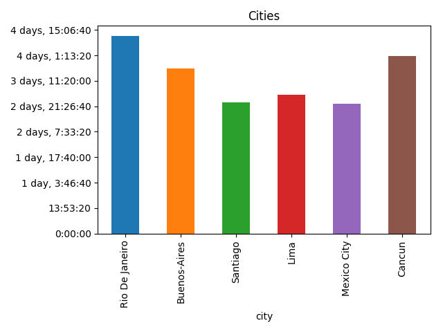
Now it’s time to work with photos. I’ve downloaded all photos from Google Photos, parsed creation dates from Exif, and “joined” them with cities by creation date:
raw_photos=pd.DataFrame(list(read_photos()),columns=['name','created_at'])# read_photos available in the gistphotos_cities=raw_photos.assign(key=0).merge(cities.assign(key=0),how='outer')photos=photos_cities[(photos_cities.created_at>=photos_cities.arrived)&(photos_cities.created_at<=photos_cities.left)]>>>photos.head()namecreated_atkeycityspentarrivedleft1photos/20180913_183207.jpg2018-09-1318:32:070Buenos-Aires3days18:00:092018-09-1223:29:522018-09-1617:30:016photos/20180909_141137.jpg2018-09-0914:11:360RioDeJaneiro4days11:55:382018-09-0811:34:142018-09-1223:29:5214photos/20180917_162240.jpg2018-09-1716:22:400Santiago2days23:24:122018-09-1617:30:012018-09-1916:54:1322photos/20180923_161707.jpg2018-09-2316:17:070MexicoCity2days22:45:222018-09-2220:43:422018-09-2519:29:0426photos/20180917_111251.jpg2018-09-1711:12:510Santiago2days23:24:122018-09-1617:30:012018-09-1916:54:13After that I’ve got the amount of photos by city:
photos_by_city=photos \
    .groupby(by='city') \
    .agg({'name':'count'}) \
    .rename(columns={'name':'photos'}) \
.reset_index()>>>photos_by_citycityphotos0Buenos-Aires1931Cancun2922Lima2953MexicoCity2564RioDeJaneiro4225Santiago267>>>photos_by_city.plot(x='city',y='photos',kind="bar",title='Photos by city',legend=False)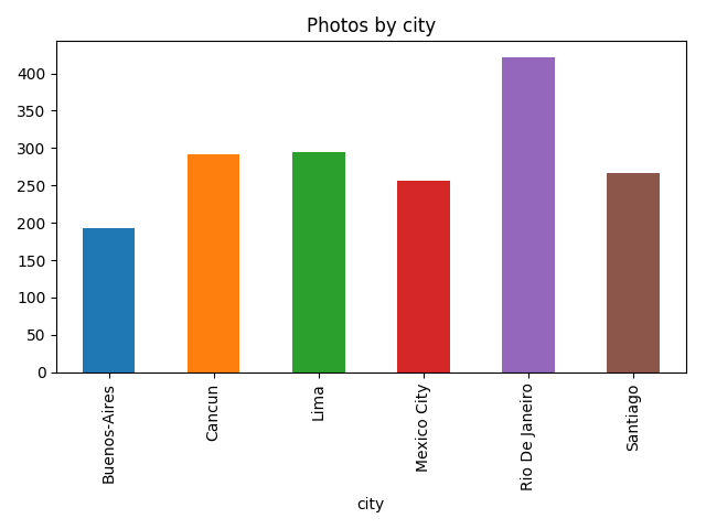
Let’s go a bit deeper and use image recognition, to not reinvent the wheel I’ve used a slightly modified version of TensorFlow imagenet tutorial example and for each photo find what’s on it:
classify_image.init()tags=tagged_photos.name\
    .apply(lambdaname:classify_image.run_inference_on_image(name,1)[0]) \
.apply(pd.Series)tagged_photos=photos.copy()tagged_photos[['tag','score']]=tags.apply(pd.Series)tagged_photos['tag']=tagged_photos.tag.apply(lambdatag:tag.split(', ')[0])>>>tagged_photos.head()namecreated_atkeycityspentarrivedlefttagscore1photos/20180913_183207.jpg2018-09-1318:32:070Buenos-Aires3days18:00:092018-09-1223:29:522018-09-1617:30:01cinema0.1644156photos/20180909_141137.jpg2018-09-0914:11:360RioDeJaneiro4days11:55:382018-09-0811:34:142018-09-1223:29:52pedestal0.66712814photos/20180917_162240.jpg2018-09-1716:22:400Santiago2days23:24:122018-09-1617:30:012018-09-1916:54:13cinema0.22540422photos/20180923_161707.jpg2018-09-2316:17:070MexicoCity2days22:45:222018-09-2220:43:422018-09-2519:29:04obelisk0.77524426photos/20180917_111251.jpg2018-09-1711:12:510Santiago2days23:24:122018-09-1617:30:012018-09-1916:54:13seashore0.24720So now it’s possible to find things that I’ve taken photos of the most:
photos_by_tag=tagged_photos \
    .groupby(by='tag') \
    .agg({'name':'count'}) \
    .rename(columns={'name':'photos'}) \
    .reset_index() \
    .sort_values('photos',ascending=False) \
.head(10)>>>photos_by_tagtagphotos107seashore27676monastery14264lakeside11686palace1153alp8681obelisk72101promontory50105sandbar4917bellcote4339cliff42>>>photos_by_tag.plot(x='tag',y='photos',kind='bar',legend=False,title='Popular tags')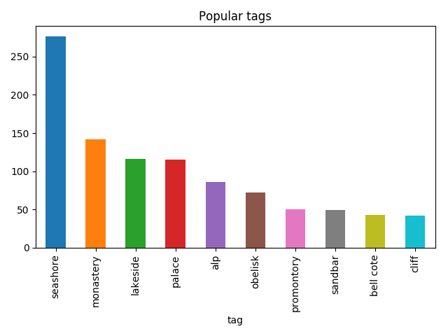
Then I was able to find what I was taking photos of by city:
popular_tags=photos_by_tag.head(5).tagpopular_tagged=tagged_photos[tagged_photos.tag.isin(popular_tags)]not_popular_tagged=tagged_photos[~tagged_photos.tag.isin(popular_tags)].assign(tag='other')by_tag_city=popular_tagged \
    .append(not_popular_tagged) \
    .groupby(by=['city','tag']) \
    .count()['name'] \
.unstack(fill_value=0)>>>by_tag_citytagalplakesidemonasteryotherpalaceseashorecityBuenos-Aires51241233010Cancun01961534110Lima025421363854MexicoCity7926197512RioDeJaneiro734517212471Santiago117271693419>>>by_tag_city.plot(kind='bar',stacked=True)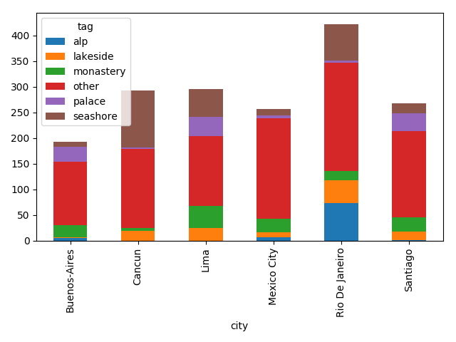
Although the most common thing on this plot is “other”, it’s still fun.