Consider the linear regression model, $$ y_i=f_i(\boldsymbol{x}|\boldsymbol{\beta})+\varepsilon_i, $$ where $y_i$ is the response or the dependent variable at the $i$th case, $i=1,\cdots, N$ and the predictor or the independent variable is the $\boldsymbol{x}$ term defined in the mean function $f_i(\boldsymbol{x}|\boldsymbol{\beta})$. For simplicity, consider the following simple linear regression (SLR) model, $$ y_i=\beta_0+\beta_1x_i+\varepsilon_i. $$ To obtain the (best) estimate of $\beta_0$ and $\beta_1$, we solve for the least residual sum of squares (RSS) given by, $$ S=\sum_{i=1}^{n}\varepsilon_i^2=\sum_{i=1}^{n}(y_i-\beta_0-\beta_1x_i)^2. $$ Now suppose we want to fit the model to the following data, Average Heights and Weights for American Women, where weight is the response and height is the predictor. The data is available in R by default.
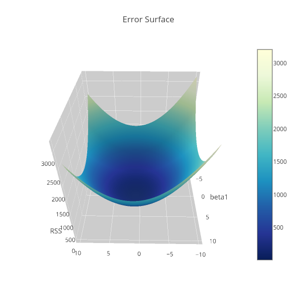
The following is the plot of the residual sum of squares of the data base on the SLR model over $\beta_0$ and $\beta_1$, note that we standardized the variables first before plotting it, If you are interested on the codes of the above figure, please click here. To minimize this elliptic paraboloid, differentiation has to be done with respect to the parameters, and then equate this to zero to obtain the stationary point, and finally solve for $\beta_0$ and $\beta_1$. For more on derivation of the estimates of the parameters see reference 1.
Formula, defined above as
The Coefficients section above returns the estimated coefficients of the model, and these are $\beta_0 = -87.51667$ and $\beta_1=3.45000$ (it should be clear that we used the unstandardized variables for obtaining these estimates). The estimates are both significant base on the p-value under .05 and even in .01 level of the test. Using the estimated coefficients along with the residual standard error we can now construct the fitted line and it's confidence interval as shown below.
Above output is the estimate of the parameters, to obtain the predicted values and plot these along with the data points like what we did in R, we can wrapped the functions above into a class called
Using this class and its methods, fitting the model to the data is coded as follows:
The predicted values of the data points is obtain using the
And Figure 2 below shows the plot of the predicted values along with its confidence interval and data points.
If one is only interested on the estimates of the model, then
Clearly, we could spare time with statsmodels, especially in diagnostic checking involving test statistics such as Durbin-Watson and Jarque-Bera tests. We can of course add some plotting for diagnostic, but I prefer to discuss that on a separate entry.
Next we fit the model to the data using the
Although we did not use intercept in simulating the data, but the obtained estimates for $\beta_1$ and $\beta_2$ are close to the true parameters (.35 and .56). The intercept, however, will help us capture the noise term we added in simulation.
Next we'll try MLR in Python using statsmodels, consider the following:
It should be noted that, the estimates in R and in Python should not (necessarily) be the same since these are simulated values from different software. Finally, we can perform MLR in SAS as follows:
The following is the plot of the residual sum of squares of the data base on the SLR model over $\beta_0$ and $\beta_1$, note that we standardized the variables first before plotting it, If you are interested on the codes of the above figure, please click here. To minimize this elliptic paraboloid, differentiation has to be done with respect to the parameters, and then equate this to zero to obtain the stationary point, and finally solve for $\beta_0$ and $\beta_1$. For more on derivation of the estimates of the parameters see reference 1.
Simple Linear Regression in R
In R, we can fit the model using thelm function, which stands for linear models, i.e.Formula, defined above as
{response ~ predictor}, is a handy method for fitting model to the data in R. Mathematically, our model is $$ weight = \beta_0 + \beta_1 (height) + \varepsilon. $$ The summary of it is obtain by running model %>% summary or for non-magrittr user summary(model), given the model object defined in the previous code,The Coefficients section above returns the estimated coefficients of the model, and these are $\beta_0 = -87.51667$ and $\beta_1=3.45000$ (it should be clear that we used the unstandardized variables for obtaining these estimates). The estimates are both significant base on the p-value under .05 and even in .01 level of the test. Using the estimated coefficients along with the residual standard error we can now construct the fitted line and it's confidence interval as shown below.
 |
| Fig 1. Plot of the Data and the Predicted Values in R. |
Simple Linear Regression in Python
In Python, there are two modules that have implementation of linear regression modelling, one is in scikit-learn (sklearn) and the other is in Statsmodels (statsmodels). For example we can model the above data using sklearn as follows: Above output is the estimate of the parameters, to obtain the predicted values and plot these along with the data points like what we did in R, we can wrapped the functions above into a class called
linear_regression say, that requires Seaborn package for neat plotting, see the codes below:Using this class and its methods, fitting the model to the data is coded as follows:
The predicted values of the data points is obtain using the
predict method, And Figure 2 below shows the plot of the predicted values along with its confidence interval and data points.
 |
| Fig 2. Plot of the Data and the Predicted Values in Python. |
LinearRegression of scikit-learn is sufficient, but if the interest on other statistics such as that returned in R model summary is necessary, the said module can also do the job but might need to program other necessary routine. statsmodels, on the other hand, returns complete summary of the fitted model as compared to the R output above, which is useful for studies with particular interest on these information. So that modelling the data using simple linear regression is done as follows:Clearly, we could spare time with statsmodels, especially in diagnostic checking involving test statistics such as Durbin-Watson and Jarque-Bera tests. We can of course add some plotting for diagnostic, but I prefer to discuss that on a separate entry.
Simple Linear Regression in SAS
Now let's consider running the data in SAS, I am using SAS Studio and in order to import the data, I saved it as a CSV file first with columns height and weight. Uploaded it to SAS Studio, in which follows are the codes below to import the data.Next we fit the model to the data using the
REG procedure,| Number of Observations Read | 15 |
|---|---|
| Number of Observations Used | 15 |
| Analysis of Variance | |||||
|---|---|---|---|---|---|
| Source | DF | Sum of Squares | Mean Square | F Value | Pr > F |
| Model | 1 | 3332.70000 | 3332.70000 | 1433.02 | <.0001 |
| Error | 13 | 30.23333 | 2.32564 | ||
| Corrected Total | 14 | 3362.93333 | |||
| Root MSE | 1.52501 | R-Square | 0.9910 |
|---|---|---|---|
| Dependent Mean | 136.73333 | Adj R-Sq | 0.9903 |
| Coeff Var | 1.11531 |
| Parameter Estimates | |||||
|---|---|---|---|---|---|
| Variable | DF | Parameter Estimate | Standard Error | t Value | Pr > |t| |
| Intercept | 1 | -87.51667 | 5.93694 | -14.74 | <.0001 |
| height | 1 | 3.45000 | 0.09114 | 37.86 | <.0001 |
Multiple Linear Regression (MLR)
To extend SLR to MLR, we'll demonstrate this by simulation. Using the formula-basedlm function of R, assuming we have $x_1$ and $x_2$ as our predictors, then following is how we do MLR in R:Although we did not use intercept in simulating the data, but the obtained estimates for $\beta_1$ and $\beta_2$ are close to the true parameters (.35 and .56). The intercept, however, will help us capture the noise term we added in simulation.
Next we'll try MLR in Python using statsmodels, consider the following:
It should be noted that, the estimates in R and in Python should not (necessarily) be the same since these are simulated values from different software. Finally, we can perform MLR in SAS as follows:
| Number of Observations Read | 100 |
|---|---|
| Number of Observations Used | 100 |
| Analysis of Variance | |||||
|---|---|---|---|---|---|
| Source | DF | Sum of Squares | Mean Square | F Value | Pr > F |
| Model | 2 | 610.86535 | 305.43268 | 303.88 | <.0001 |
| Error | 97 | 97.49521 | 1.00511 | ||
| Corrected Total | 99 | 708.36056 | |||
| Root MSE | 1.00255 | R-Square | 0.8624 |
|---|---|---|---|
| Dependent Mean | 244.07327 | Adj R-Sq | 0.8595 |
| Coeff Var | 0.41076 |
| Parameter Estimates | |||||
|---|---|---|---|---|---|
| Variable | DF | Parameter Estimate | Standard Error | t Value | Pr > |t| |
| Intercept | 1 | 18.01299 | 11.10116 | 1.62 | 0.1079 |
| X1 | 1 | 0.31770 | 0.01818 | 17.47 | <.0001 |
| X2 | 1 | 0.58276 | 0.03358 | 17.35 | <.0001 |
Conclusion
In conclusion, SAS saves a lot of work, since it returns complete summary of the model, no doubt why companies prefer to use this, besides from their active customer support. R and Python, on the other hand, despite the fact that it is open-source, it can well compete with the former, although it requires programming skills to achieved all of the SAS outputs, but I think that's the exciting part of it -- it makes you think, and manage time. The achievement in R and Python is of course fulfilling. Hope you've learned something, feel free to share your thoughts on the comment below.Reference
- Draper, N. R. and Smith, H. (1966). Applied Regression Analysis. John Wiley & Sons, Inc. United States of America.
- Scikit-learn Documentation
- Statsmodels Documentation
- SAS Documentation
- Delwiche, Lora D., and Susan J. Slaughter. 2012. The Little SAS® Book: A Primer, Fifth Edition. Cary, NC: SAS Institute Inc.
- Regression with SAS. Institute for Digital Research and Education. UCLA. Retrieved August 13, 2015.
- Python Plotly Documentation


