John Cook: How to create Green noise in Python

This is a follow-on to my previous post on green noise. Here we create green noise with Python by passing white noise through a Butterworth filter.

Green noise is in the middle of the audible spectrum (on the Bark scale), just where our hearing is most sensitive, analogous to the green light, the frequency where our eyes are most sensitive. See previous post for details, including an explanation of where the left and right cutoffs below come from.

Here’s the code:

from scipy.io.wavfile import write
from scipy.signal import buttord, butter, filtfilt
from scipy.stats import norm
from numpy import int16

def turn_green(signal, samp_rate):
    # start and stop of green noise range
    left = 1612 # Hz
    right = 2919 # Hz

    nyquist = (samp_rate/2)
    left_pass  = 1.1*left/nyquist
    left_stop  = 0.9*left/nyquist
    right_pass = 0.9*right/nyquist
    right_stop = 1.1*right/nyquist

    (N, Wn) = buttord(wp=[left_pass, right_pass],
                      ws=[left_stop, right_stop],
                      gpass=2, gstop=30, analog=0)
    (b, a) = butter(N, Wn, btype='band', analog=0, output='ba')
    return filtfilt(b, a, signal)

def to_integer(signal):
    # Take samples in [-1, 1] and scale to 16-bit integers,
    # values between -2^15 and 2^15 - 1.
    signal /= max(signal)
    return int16(signal*(2**15 - 1))

N = 48000 # samples per second

white_noise= norm.rvs(0, 1, 3*N) # three seconds of audio
green = turn_green(white_noise, N)
write("green_noise.wav", N, to_integer(green))

And here’s what it sounds like:

(download .wav file)

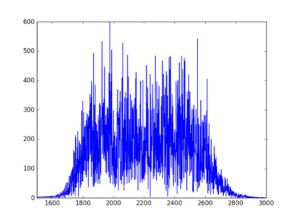
Let’s look at the spectrum to see whether it looks right. We’ll use one second of the signal so the x-axis coincides with frequency when we plot the FFT.

from scipy.fftpack import fft

one_sec = green[0:N]
plt.plot(abs(fft(one_sec)))
plt.xlim((1500, 3000))
plt.show()

Here’s the output, concentrated between 1600 and 3000 Hz as expected: