Tweet Sentiment Analysis Using LSTM With PyTorch

We will go through a common case study (sentiment analysis) to explore many techniques and patterns in Natural Language Processing.

Overview:

• Imports and Data Loading
• Data Preprocessing
  • Null Value Removal
  • Class Balance
• Tokenization
• Embeddings
• LSTM Model Building
• Setup and Training
• Evaluation

Imports and Data Loading

This dataset can be found on Github in this repo: https://github.com/ajayshewale/Sentiment-Analysis-of-Text-Data-Tweets-

It is a sentiment analysis dataset comprised of 2 files:

• train.csv, 5971 tweets
• test.csv, 4000 tweets

The tweets are labeled as:

• Positive
• Neutral
• Negative

Other datasets have different or more labels, but the same concepts apply to preprocessing and training. Download the files and store them locally.

Before working with PyTorch, make sure to set the device. This line of code selects a GPU if available.

Since the data is stored in csv files, we can use the pandas function .read_csv() to parse both train and test files:

Data Preprocessing

Null Value Removal

After parsing the files, it is important to analyze the text to understand the preprocessing steps you will take.

Preprocessing is about cleaning the files from inconsistent, useless, or noisy information. So, we first look for things to remove.

• We can see a few tweets that are "Not Available", and they will not help train our model.
• Also, the column "Id" is not useful in machine learning, since the ID of a tweet does not affect its sentiment.
• We may not see any in the sample displayed, but there may be null values (NaN) in the columns. Pandas has a function .dropna() that drops null values.

So far so good, let us take a look at the test set:

It turns out that the test set unfortunately has no Category column. Thus, it will not be very useful for us. However, we can do some preprocessing for pratice:

• The tweets column is wrongly named "Category", we can rename it:

Then, we apply the same steps as we did on the train set.

Class Imbalance

Next, since this is a classification task, we must make sure that the classes are balanced in terms of number of instances. Otherwise, any model we train will be skewed and less accurate.

First, we find the counts of each class:

Supervised datasets typically have balanced classes. However, as seen in this dataset, the number of positive and neutral tweets are a lot more than the negative tweets. There are several solutions to fix imbalance problem:

• Oversampling
• Undersampling
• Hybrid approaches
• Augmentation

Oversampling

To re-adjust the class imbalance, in oversampling, you duplicate some tweets in the minority classes until you have similar number of tweets for each class. So for example, we would duplicate the negative set ~3 times to acquire 2600 negative tweets. We can also do the same for neutral tweets. By doing so, you end up with all classes having 2600 tweets.

Undersampling

In undersampling, instead of increasing the number of tweets in the minority classes, you decrease the number of tweets in the majority classes. You do so simply by deleting tweets in the majority classes randomly until you have 869 tweets in all classes.

Hybrid Approaches

Both oversampling and undersampling can be a bit extreme. One can do a mixture of both by determining a final number of tweets that is between the minimum and the maximum. For instance, we can select 2000 as the final tweet count. Then, we delete ~600 positive tweets, keep neutral tweets the same, and duplicate the negative tweets by a factor of ~2.3. This way we end up with ~2000 tweets in each class.

Augmentation

Augmentation is more complex than the other approaches. In augmentation, you use the existing negative tweets to create new negative tweets. By doing so, you can increase the number of negative and neutral tweets until they are all 2600.

It is a relatively new concept, but you can find more about it in the papers listed here: https://paperswithcode.com/task/text-augmentation/codeless

For our purpose, we undersample positive and neutral classes till we have 869 tweets in each class. We are doing undersampling manually in this excercise, but there is a python library called imblearn that can perform under/oversampling.

After undersampling both neutral and positive classes, we join them all together again:

As shown, the value counts have been adjusted.

Moving forward, since we do not have a labeled test set, we split the train set into train and test sets with ratios of 85:15

Since the data is small, we can transfer them into python lists for further manipulation. If the data is large, it's preferred to keep using pandas until you create the batch iterator (DataLoader in PyTorch).

We can observe that some tweets end with links. Moreover, we can see that many tweets have twitter mentions (@someone). These are not useful in determining the sentiment of the tweet, and it is better to remove them before proceeding:

As showm, regex can remove such strings easily. Finally, notice that we lowercased all tweets in the function. The simple reason is that for a computer, case differences are important. For example, the word "word" and "Word" are as different as any other 2 pairs of words, although for us they are the same. To improve training, it is better to lowercase all words.

Tokenization

Finally, using word_tokenize() from the NLTK library, we can split the sentence into tokens, or words, puncatation points, and other language blocks that are "divisbile".

Next, we create the "vocabulary" of the corpus. In NLP projects, the vocabulary is just a mapping of each word to a unique ID. Since models cannot process text as we do, we must convert them into numerical form.

By creating this mapping, one can write a sentence with numbers. For instance, if the vocab is as follows:

{"i": 0,
 "the: 1,
 "ate": 2,
 "pizza": 3
}

We can say "I ate the pizza" by saynig [0, 2, 1, 3].

This is an oversimplified explanation of encoding, but the general idea is the same.

In this exercise, we create a list of unique words (set-like) and use that list and its indices to create a dictionary of mapping.

As shown, the list starts with the 3 tokens "<PAD>", "<SOS>", "<EOS>".

Since we will input fixed-size text to the model, we will have to pad some tweets to increase their length. The token for padding is <PAD>.

<SOS> and <EOS> are short for "start of sentence" and "end of sentence" respectively. They are tokens used to identify the beginning and ending of each sentence in order to train the model. As will be showm, they will be inserted at the beginning and end of every tweet

As shown, index2word and word2index act as our vocabulary which can be used to encode all tweets.

ALso, we cannot leave the labels in text form. So, we encode them using 0, 1, and 2 for negative, neutral, and positive respectively.

To pad, we must select a sequence length. This length should cover the majority of tweets. Typically, length measurements are performed to find the ideal sequence length, but since our data is tweet data im 2012, we know that they cannot be too long and therefore we can set the length to 32 tokens.

Then, we perform padding and truncating. Padding is performed when a tweet is shorter than 32 tokens, and truncating is used when a tweet is longer than 32 tokens. In the same encoding method, we also insert the PAD, SOS, and EOS tokens.

Encoding both train and test sets:

This is what 3 tweets look like after encoding:

Notice that they always begin with 1, which stands for SOS, and end with 2, which is EOS. If the tweet is shorter than 32 tokens, it is then padded with 0's, which is the padding. Also, notice that the labels are numerical as well.

Now, the data is preprocessed and encoded. It is time to create our PyTorch Datasets and DataLoaders:

Notice the parameter drop_last=True. This is used for when the final batch does not have 50 elements. The batch is then incomplete and will cause dimension errors if we feed it into the model. By setting this parameter to True, we avoid this final batch.

PyTorch LSTM Model Buidling

Building LSTMs is very simple in PyTorch. Similar to how you create simple feed-forward neural networks, we extend nn.Module, create the layers in the initialization, and create a forward() method.

In the initialization, we create an embeddings layer first.

Embeddings are used for improving the representation of the text. This Wikipedia article explains embeddings well: https://en.wikipedia.org/wiki/Word_embedding#:~:text=In%20natural%20language%20processing%20.

In short, instead of feeding sentences as simple encoded sequences (for example [0, 1, 2], etc. as seen in the pizza example), we can improve the representation of every token.

Word embeddings are vectors that represent each word, instead of a single number in the pizza example.

Why does a vector help? Vectors allow you to highlight the similarities between words. For instance, we can give the words "food" and "pizza" similar vectors since the 2 words are related. This makes it easier for the model to "understand" the text.

As seen, in PyTorch it is a simple layer, and we only need to feed the data into it. Vectors are initially initialized randomly for every word, and then adjusted during training. That means that the embeddings are trainable parameters in this network.

Another alternative to using random initialization is to use pre-trained vectors. Big AI labs at Google, Facebook, and Stanford have created pre-trained embeddings that you can just download and use. They are called word2vec, fastText, and GloVe respectively.

This is a good example of how to use pre-trained embeddings such as word2vec in the Embedding layer of PyTorch: https://medium.com/@martinpella/how-to-use-pre-trained-word-embeddings-in-pytorch-71ca59249f76

Finally, as seen, we have an init_hidden() method. The reason we need this method is that at the beginning of the sequence, there are no hidden states.

The LSTM takes in initial hidden states of zeros at the first time-step. So, we initalize them using this method.

Now, we initialize the model and move it to device as follows:

Setup and Training

Next, we create the criterion and optimizer used for training:

Then we train the model for 50 epochs:

We plot the loss at each batch to make sure that the mode is learning:

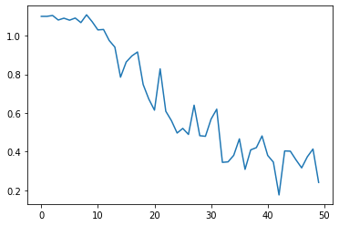
As shown, the losses are decreasing steadily and then they level off, which means that the model has successfully learnt what can be learned from the data.

To test the model, we run the same loop for the the test set and extract the accuracy:

Evaluation

While this is generally a low accuracy, it is not insignificant. If the model did not learn, we would expect an accuracy of ~33%, which is random selection.

However, since the dataset is noisy and not robust, this is the best performance a simple LSTM could achieve on the dataset.

According to the Github repo, the author was able to achieve an accuracy of ~50% using XGBoost.

Conclusion

In this tutorial, we created a simple LSTM classifier for sentiment analysis. Along the way, we learned many NLP techniques used in real NLP projects. While the accuracy was not as high as accuracies for other datasets, we can conclude that the model learned what it could from the data, as shown by the loss.